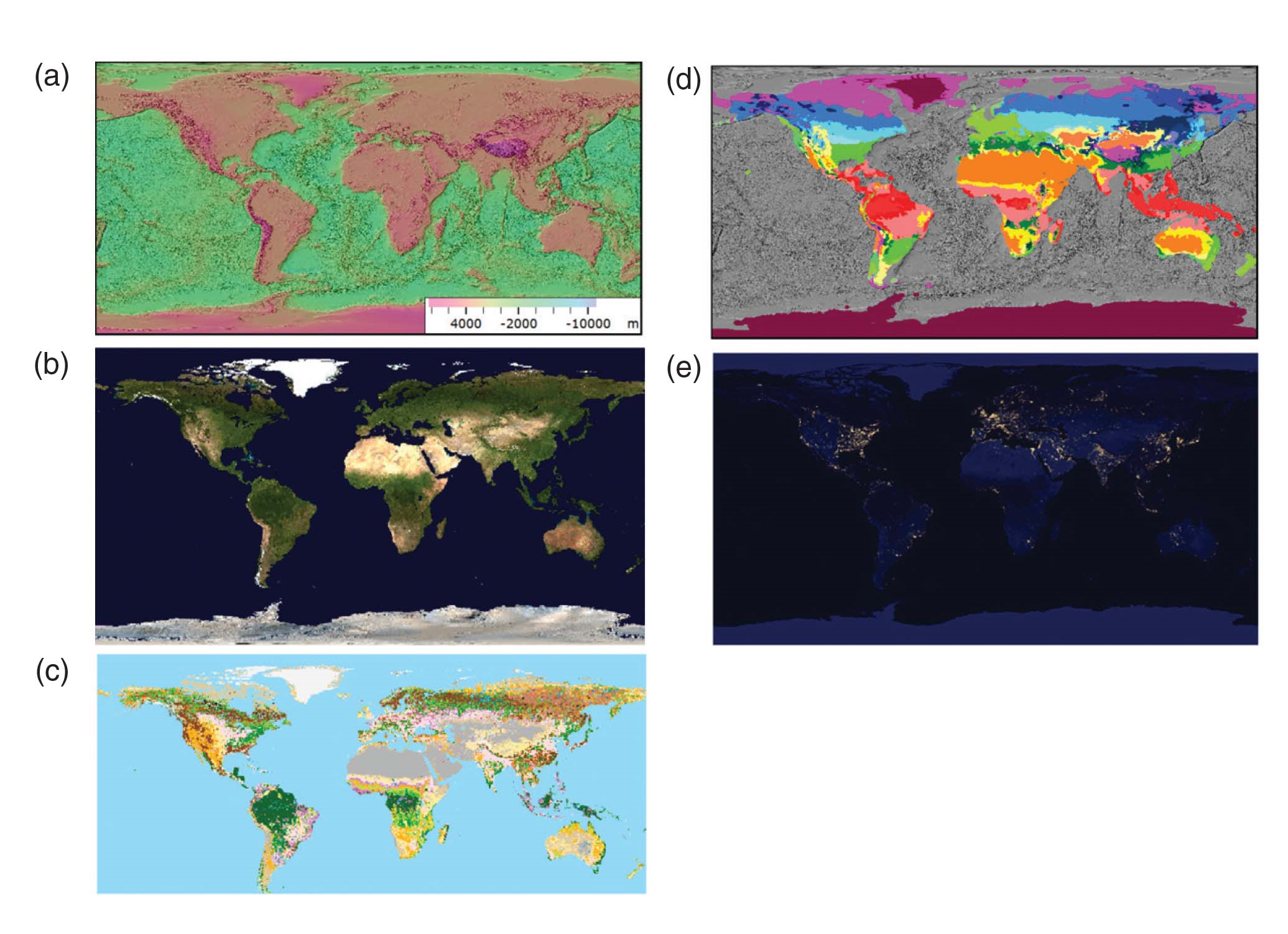
Global terrain analysis: (a) topography; (b) cloud-free composite satellite imagery; (c) global land cover; (d) Köppen-Geiger climate classification; and (e) night lights

Harpers Ferry, West Virginia, from a 1/3” NED DEM: (a) hillshade combined with colours for elevation; (b) greyscale hillshade with TIGER roads, streams and railroads in cyan; (c) greyscale hillshade combined with geologic map (Southworth et al., 2000); (d) elevations displayed with colour and greyscale

Maps of part of the 1/3” NED DEM near Harpers Ferry, United States. Five maps use focal operations (hillshade, slope, aspect, and two convexities), while three use zonal operations (relief and two openness measures) which require definition of a 1000 m region.

Landform classification performed in WhiteBox Tools, exported as a Geotiff to MICRODEM, and exported as KMZ to Google Earth. The irregular white collar is a result of reprojecting the UTM data from WhiteBox Tools into the geographic projection required for Google Earth.

Six views of a lidar point cloud from Keene, New Hampshire. (a) east–west one-metre-thick slice; (b) one-metre DSM created from the data; (c) one-metre DTM; and (d) 3D view of the point cloud; (e) maps showing points coloured by elevation; (f) return intensity, and (g) classification.

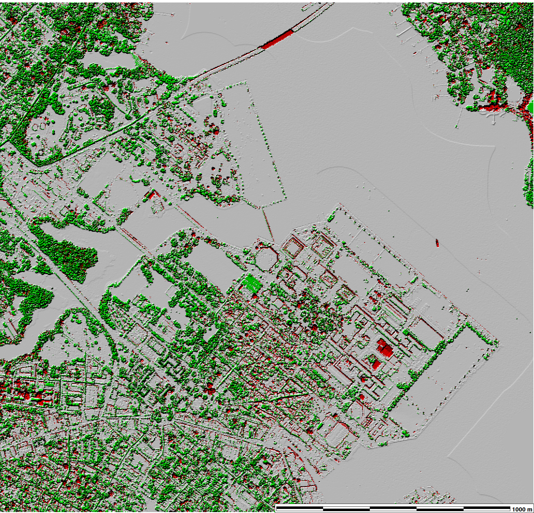
Lidar detected changes between 2011 and 2017 for the US Naval Academy. Red colours were 2 or more metres lower in 2011, while green colours were two of more metres higher