An Adventure in Statistics: The Reality Enigma
Student Resources
Jig:Saw’s puzzle solutions
Puzzle 1
Earlier in his journey, Milton tried to convince Zach that trying to learn statistics dressed as Florence Nightingale would help him (Chapter 8). This intervention was based on research by Zhang et al. (2013) showing that women completing a maths test under a fake name performed better than those using their real name. Table 15.5 (in the book and reproduced below) has a random selection of the scores from that study. The table shows scores from 20 women and 20 men; in each case half performed the test using their real name whereas the other half used a fake name. Conduct an analysis on the women’s data to see whether scores were significantly higher for those using a fake name compared to those using their own name.
Table 15.5 (reproduced): A random selection of data from Zhang et al. (2013). Scores show the percentage correct on a maths test when males and females take the test either using their own name, or a fake name.

Whether someone conducted the maths test using their own name or a fake name is represented by the variable Name, and we want to predict this variable from Score, which is how well the person scored on the maths test. The model can be expressed as follows:
![]()
Because the experiment in this puzzle uses different entities in each group (i.e. different women took part in the fake-name and own-name conditions), the design is known as an independent design and therefore requires us to conduct an independent t-test. We could assign participants who took the maths test under their own name a value of 0 for the variable Name; this is the baseline group. The ‘experimental’ group was made up of participants who took the test under a fake name, and we could assign these participants a value of 1 for the variable Name.
Table 1: Calculating cross-product deviations
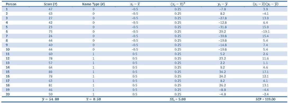
We need to calculate estimates for b0 and b1 in the model. To compute b1, we calculate the total relationship between the predictor and outcome, the sum of cross-products (SCP) and divide this value by the total deviation of the predictor from its mean, SSx (you can find these values in Table 1):
![]()
We could also calculate b1 by taking the difference between the two group means (you can find the means in Table 15.5 (reproduced)):
![]()
![]()
Calculating b0 is easy because it is equal to the mean of the baseline group (the group that we coded as 0), which in this case was the own-name group:
![]()
or:

Next we need to calculate the sum of squared residuals, which I have done in Table 2. I calculated the sum of squared residuals to be 4317.00 and we can turn this total error into an average by dividing by the degrees of freedom. The degrees of freedom will be N-p, where p is the number of parameters. There were 20 participants, N, and two parameters (b0 and b1), so we divide the residual sum of squares, 4317.00, by 20-2, which is 18. The resulting mean squared error in the model is 239.83.
![]()
The standard error of the model will then be the square root of this value:

Table 2: Calculating the sum of squared residuals
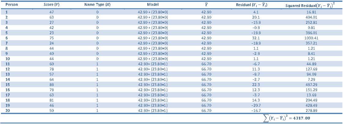
We can then use the standard error in the model to calculate the standard error for the b by dividing by the square root of the sum of squares for the predictor (sum of cross-products) (see Table 1):
![]()
We can now calculate the t-value:
![]()
Now we need to look up the critical value for t (see the table ‘Critical values of the t-distribution’ at the back of the main textbook) at the 0.05 significance level with 18 degrees of freedom, which is 2.10. Our observed value of 3.44 is larger than the critical value, indicating that we have a significant result. In other words, we can conclude that scores on the maths test were significantly different in females who used their own name compared to females who used a fake name, and the means tell us that women who used a fake name scored significantly higher on the maths test than women who used their own name.
Puzzle 2
Conduct the same analysis as above but on the male participants.
For this puzzle we will follow the same procedure as in puzzle 1, only using the data for the male participants in Table 15.5 rather than the data for the female participants. The model will therefore be the same:
![]()
The experiment in this puzzle again uses different entities in each group (i.e. different men took part in the fake-name and own-name conditions), so again we have an independent design, which requires us to conduct an independent t-test.
When we conducted this test on the female participants (puzzle 1) we assigned participants who took the maths test under their own name a value of 0 for the variable Name (the baseline group), and participants who took the test under a fake name (the experimental group) a value of 1 for the variable Name, and we can do the same for the male participants.
Table 3: Calculating cross-product deviations
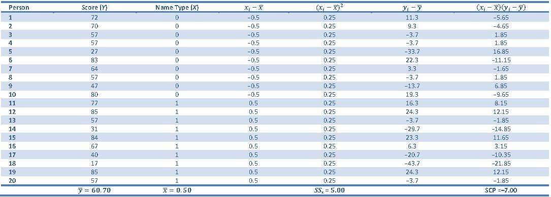
As in the previous puzzle, we first need to calculate estimates for b0 and b1 in the model. To compute b1, we calculate the total relationship between the predictor and outcome, the sum of cross products (SCP) and divide this value by the total deviation of the predictor from its mean, SSx (you can find these values in Table 3):
![]()
A far easier way of calculating b1 would be to calculate the difference between the two group means (you can find the means in Table 15.5 (reproduced)):
![]()
![]()
Calculating b0 is easy because it is equal to the mean of the baseline group (the group that we coded as zero), which in this case was the own-name group:
![]()
or

Next we need to calculate the sum of squared residuals, which I have done in Table 4. I calculated the sum of squared residuals to be 7726.40, and we can turn this total error into an average by dividing by the degrees of freedom. The degrees of freedom will be N-p, where p is the number of parameters. There were 20 participants, N, and two parameters (b0 and b1), so we divide the residual sum of squares, 7726.40, by 20-2, which is 18. The resulting mean squared error in the model is 429.24.
![]()
The standard error of the model will then be the square root of this value:

Table 4: Calculating the sum of squared residuals
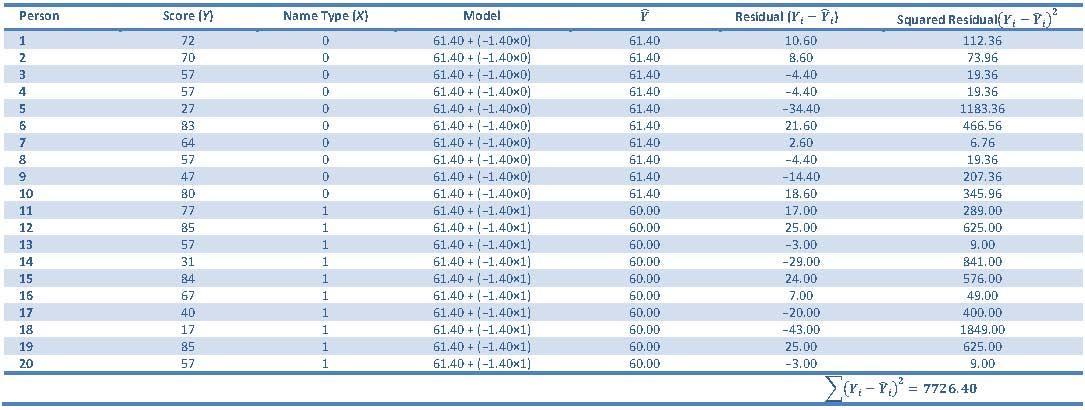
We can then use the standard error in the model to calculate the standard error for the b by dividing by the square root of the sum of squares for the predictor (sum of cross-products) (see Table 3):
![]()
We can now calculate the t-value:
![]()
Now we need to look up the critical value for t (see the table ‘Critical values of the t-distribution’ at the back of the main textbook) at the 0.05 significance level with 18 degrees of freedom, which is 2.10. Our observed value of −0.15 is smaller than the critical value, indicating that we do not have a significant result. In other words, scores on the maths test were not significantly different in men who used their own name compared to men who used a fake name.
Puzzle 3
Using the analyses in puzzles 1 and 2, calculate the Cohen’s ds for the effect of using a fake vs. own name for both males and females.
Let’s start with calculating Cohen’s d for the female data. I will calculate Cohen’s d using the pooled standard deviation to give you some practice. The two groups both contained 10 participants so the Ns will both be 10. The variances for the fake-name and own-name groups are in Tables 5 and 6 respectively, and if you work all of that out the pooled standard deviation is 14.69.
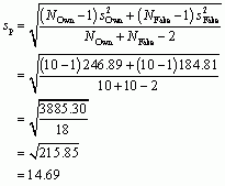
Table 5: Calculating the standard deviation of the fake-name group

Table 6: Calculating the standard deviation of the own-name group

We then use the pooled standard deviation (sp) to calculate d using the following equation:
![]()
So we end up with an effect size of 1.62. In other words, in the female data, scores in the fake-name condition were 1.62 standard deviations higher than the own-name condition, which is a large effect.
Next we can calculate Cohen’s d for the male data in exactly the same way. I will use the pooled standard deviation (sp) again and so we need to calculate this first, but before we can do that we need to calculate the variances of both the fake-name and own-name groups for the male data which I have done in Tables 7 and 8, respectively.
Table 7: Calculating the standard deviation of the fake-name group

Table 8: Calculating the standard deviation of the own-name group

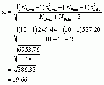
We can now calculate d using the equation:
![]()
So we end up with an effect size of −0.07. In other words, in the male data, scores in the fake-name condition were 0.07 of a standard deviation lower than the own-name condition, although this is a very small effect.
Puzzle 4
Outputs 15.7 and 15.8 (in the book and reproduced below) show Bayesian analyses of the female and male data from Table 15.5 (in the book an reproduced in puzzle 1). Interpret these outputs.
For the female data (Output 15.7) the Bayes factor is 12.92, which means that the data are 12.92 times more likely given the alternative hypothesis than they are given the null hypothesis, which would be regarded by Jeffreys as ‘strong evidence’ for the alternative hypothesis, i.e., that women score higher on a maths test when using a fake name compared to their own name. Output 15.7 also shows that the Bayesian estimate, assuming that the alternative hypothesis is true, of the difference between means (beta) is 19.836 with a standard error of 0.248. You can also use the 2.5% and 97.5% quantiles as the limits of the 95% credible interval for that difference. Again, assuming the alternative hypothesis is true, there is a 95% probability that the difference between means is somewhere between 2.44 and 34.21.
For the male data (Output 15.8) the Bayes factor is 0.40, which is less than 1 and therefore supports the null hypothesis (that there is no difference in test scores in men who used their own name compared to those who used a fake name) by suggesting that the probability of the data given the null is higher than the probability of the data given the alternative hypothesis. The output also shows that the Bayesian estimate, assuming that the alternative hypothesis is true, of the difference between means (beta) is −0.561 with a standard error of 0.243. You can also use the 2.5% and 97.5% quantiles as the limits of the 95% credible interval for that difference. Again, assuming the alternative hypothesis is true, there is a 95% probability that the difference between means is somewhere between −16.79 and 15.44.
Bayes factor analysis
--------------
[1] Alt., r=0.707 : 12.9241 ±0%
Against denominator:
Null, mu1-mu2 = 0
---
Bayes factor type: BFindepSample, JZS
1. Empirical mean and standard deviation for each variable,
plus standard error of the mean:
Mean SD Naive SE Time-series SE
mu 54.838 3.7842 0.11967 0.11967
beta (Fake - Own) 19.836 7.8554 0.24841 0.29969
2. Quantiles for each variable:
2.5% 25% 50% 75% 97.5%
mu 46.7436 52.5273 54.902 57.282 61.96
beta (Fake - Own) 2.4448 15.1047 20.140 24.759 34.21
Output 15.7: Abridged Bayes factor output for the female data in Table 15.5
Bayes factor analysis
--------------
[1] Alt., r=0.707 : 0.4006056 ±0%
Against denominator:
Null, mu1-mu2 = 0
---
Bayes factor type: BFindepSample, JZS
1. Empirical mean and standard deviation for each variable,
plus standard error of the mean:
Mean SD Naive SE Time-series SE
mu 60.59589 4.7344 0.14971 0.14971
beta (Fake - Own) -0.56118 7.6947 0.24333 0.24333
2. Quantiles for each variable:
2.5% 25% 50% 75% 97.5%
mu 51.20770 57.8040 60.55002 63.5746 70.3617
beta (Fake - Own) -16.78788 -5.2981 -0.28806 4.0389 15.4411
Output 15.8: Abridged Bayes factor output for the male data in Table 15.5
Puzzle 5
Based on puzzles 1–4 what can you conclude about the difference between males and females in the effect of taking a test using a fake name or your own name?
The analyses conducted in puzzles 1–4 (t-tests, Cohen’s ds and Bayes factor analyses) all indicate that women using a fake name tend to score higher on a maths test than those using their own name, but men achieve similar scores whether they use a fake name or their own name.
Puzzle 6
Use the analyses in puzzles 1 and 2 to write out the separate linear models for males and females that describe how accuracy scores are predicted from the type of name used. In these models, what do the b1 and b0 represent?
Let’s start with the females. As the question states, we are asking how well we can predict accuracy scores on a maths test based on whether participants used their own name or a fake name. This is a linear model with one dichotomous predictor:
![]()
We can replace the outcome, Y, with what we measured, accuracy scores (I called this variable Score) and replace the predictor, X, with the group to which a person belonged (I called this variable Name). The variable Name is a dichotomous variable – in other words, a nominal variable with two categories. We can’t put words into a statistical model so we must convert these two categories into numbers. In puzzle 1 I used dummy coding and coded women who used their own name as 0 for the variable Name and women who used a fake name as 1 for the variable Name:
![]()
In our model, b0 tells us the accuracy score when the predictor is 0, i.e., it tells us the accuracy score when a woman used her own name (because I coded ‘own name’ as 0), and b1 shows the relationship between the predictor (type of name used) and outcome (accuracy scores). We can replace the values of b0 and b1 with those that we calculated in puzzle 1:
![]()
We can then use the model to predict accuracy scores in women who used their own name by replacing Name in the equation with 0. The answer is 42.90, and if you look back at puzzle 1 you will see that this was also the mean score of the own-name group:
![]()
To predict accuracy scores in women who used a fake name we replace Name in the equation with 1. The answer is 66.70, and if you look back at puzzle 1 you will see that this was also the mean score of the fake-name group:

We can then do the same for the male participant data. The model would be the same as for females:
![]()
In the model above, b0 tells us the accuracy score when the predictor is 0, i.e., it tells us the accuracy score when a man used his own name (because I coded ‘own name’ as zero), and b1 shows the relationship between the predictor (type of name used) and outcome (accuracy scores). We can replace the values of b0 and b1 with those that we calculated in puzzle 2:
![]()
We can then use the model to predict accuracy scores in men who used their own name by replacing Name in the equation with 0 (because I coded ‘own name’ as 0). The answer is 61.40, and if you look back at puzzle 2 you will see that this was also the mean score of the own-name group:
![]()
To predict accuracy scores in men who used a fake name we can replace Name in the equation with 1 (because I coded ‘fake name’ as 1). The answer is 60.00, and if you look back at puzzle 2 you will see that this was also the mean score of the fake-name group.

Puzzle 7
Alice’s research for JIG:SAW (Alice’s Lab Notes 15.1 in the book) built upon a study by Hogarth et al. (2104) that showed that a calcite cloak could obscure what was behind it. Table 15.6 (in the book and reproduced below) shows the recognition scores for 10 participants in their study who had to recognize 20 objects hidden behind either a transparent cloak (the control) or a similar transparent cloak containing calcite. Carry out an analysis to see whether recognition scores were lower when objects were concealed by the control cloak or the calcite one.
Table 15.6 (reproduced): Data for 10 participants in Hogarth et al.’s (2104) experiment.
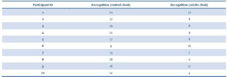
To answer this puzzle we need to conduct a paired-samples t-test because the same participants took part in both conditions of the experiment (control cloak and calcite cloak).
First we need to calculate the difference scores, the mean difference score and the standard deviation, which I have done in Table 9.
Table 9: Calculating difference scores

We can see from Table 9 that the mean is −6.80 and the standard deviation is 6.63. This suggests that, on average, people recognize fewer objects when they are obscured by a transparent cloak containing calcite than when they are obscured by a transparent cloak that does not contain calcite.
Now we need to calculate the standard error of differences, which will tell us how widely we can expect difference scores to be across samples. We can calculate the standard error of differences using the following equation:
![]()
We can now calculate the t-value by dividing the mean difference by the standard error of differences as I have done in the equation below:
![]()
If we look up the critical value for t at the 0.05 significance level with 9 (N – 1) degrees of freedom, we can see that it is 2.262. Our observed t of −3.24 is bigger than the critical value (we can ignore the minus sign as that just tells us the direction of the effect), indicating a significant result. In other words, people recognized significantly fewer objects when they were concealed by a transparent cloak containing calcite than when they were concealed by a similar transparent cloak that did not contain calcite.
Puzzle 8
What is the effect size for the effect of calcite on recognition compared to the control?
Remember that we are dealing with difference scores when we compute the test statistic. One very simple way to standardize the difference between means is to use the difference scores instead of the raw scores:
![]()
So we end up with an effect size of −1.45. In other words, recognition in the calcite condition was −1.45 standard deviations higher than in the control condition, or you might say recognition in the control condition was 1.45 standard deviations higher than in the calcite condition.
Puzzle 9
Output 15.9 (in the book and reproduced below) shows a Bayesian analysis of the recognition scores from Table 15.6. Interpret the output.
The Bayes factor is 6.15, which means that the data are 6.15 times more likely under the alternative hypothesis compared to under the null, which would be regarded by Jeffreys as ‘evidence with substance’ for the alternative hypothesis, i.e., that a cloak containing calcite decreases recognition scores when compared to a control cloak. The difference between means is estimated as 5.87, and there is a 95% probability that the effect lies between 1.41 and 10.63, assuming the alternative hypothesis is true.
Bayes factor analysis
--------------
[1] Alt., r=0.707 : 6.148254 ±0%
Against denominator:
Null, mu = 0
---
Bayes factor type: BFoneSample, JZS
1. Empirical mean and standard deviation for each variable,
plus standard error of the mean:
Mean SD Naive SE Time-series SE
mu 5.8705 2.3628 0.07472 0.08214
2. Quantiles for each variable:
2.5% 25% 50% 75% 97.5%
mu 1.4121 4.3430 5.8204 7.300 10.631
Output 15.9: Abridged Bayes factor output for the data in Table 15.6
Puzzle 10
What are the 95% credible intervals in Outputs 15.7, 15.8, and 15.9? What is the difference between a confidence interval and a credible interval?
Looking at Outputs 15.7, 15.8, and 15.9, you can use the 2.5% and 97.5% quantiles as the limits of the 95% credible interval for the difference between means. So assuming the alternative hypothesis is true, there is a 95% probability that the difference between means is somewhere between 2.44 and 34.21 in Output 15.7, a 95% probability that the difference between means is somewhere between −16.79 and 15.44 in Output 15.8, and a 95% probability that the difference between means is somewhere between 1.41 and 10.63 in Output 15.9.
A confidence interval is set so that before the data are collected there is a 95% chance that the interval will contain the true value of the parameter. Once the data are collected, your sample is either one of the 95% that produce an interval containing the true value, or it is one of the 5% that do not. In other words, having collected the data, the probability of the interval containing the true value of the parameter is either 0 (it does not contain it) or 1 (it does contain it), but you do not know which. A credible interval is different in that it reflects the plausible probability that the interval contains the true value. For example, a 95% credible interval has a 0.95 probability of containing the true value; this is not true of a 95% confidence interval (the probability of it containing the true value is either 0 or 1, but you don’t know which).
You cannot use a credible interval to test hypotheses because it is constructed assuming that the alternative hypothesis is true. It tells you the interval within which the effect will fall with 95% probability, assuming that the effect exists. It tells you nothing about the null hypothesis.
