A robust estimate is one that is reliable even when the normal assumptions of the statistic are not met.

They both give robust estimates, but the trimmed mean is the mean based on scores that have had a percentage of extreme scores removed. For example, removing the highest and lowest 20% of scores and then computing the mean of the remaining scores would give us the 20% trimmed mean. Winsorizing data, on the other hand, is where a percentage of the highest scores are replaced with the next highest score (rather than being discarded) in the data and the same percentage of the lowest scores are replaced with the next lowest score in the data.

First, let’s calculate the mean by adding the scores and dividing by the number of scores:

To trim 20% of the data from the two ends of the distribution, we need to trim 2 scores from each end (because 20% of 10 is 2). The mean of the remaining 6 scores is the 20% trimmed mean. We first need to arrange the scores in ascending order: 11, 11, 12, 13, 13, 14, 15, 15, 16, 21. Then we trim (i.e. delete) 2 scores from each end. The data are now: 12, 13, 13, 14, 15, 15 (note that we trimmed the two 11s from the bottom, and the 16 and 21 from the top). Finally, we calculate the mean of these 6 scores:

To trim 10% of the data, we need to trim 1 score from each end because 10% of 10 is 1. This involves removing the lowest score (11) and highest score (21). The remaining 8 scores are: 11, 12, 13, 13, 14, 15, 15, 16. The 10% trimmed mean will be the mean of these scores:

To calculate the 20% winsorized mean, we need to replace the top and bottom 20% of scores with the next highest or lowest score. For these data, the top 2 scores (16 and 21) are both replaced with the next highest score (15), and the bottom two scores (11 and 11) are replaced with the next lowest score (12). So the data becomes: 12, 12, 12, 13, 13, 14, 15, 15, 15, 15. We then calculate the mean of these data:

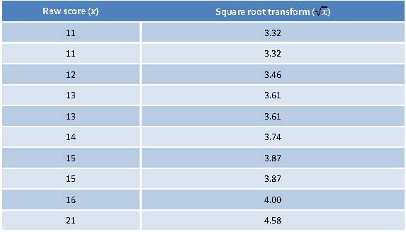
To square root transform the scores we replace each score with its square root (see Table 1).

Table 1: Raw scores and their square roots

To calculate the mean strength, we need to add up all the scores in each group and then divide the total by the number of scientists in each group.

Table 9.3 (reproduced): Scientists’ strength scores for JIG:SAW employees and non-employees (see Figure 9.1 in the book)

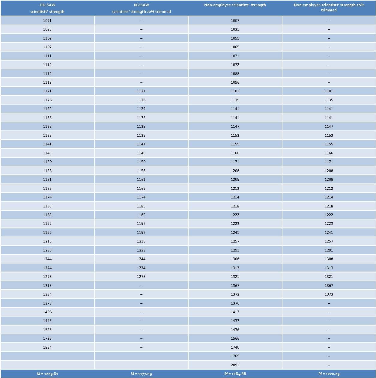
First, we will calculate the 20% trimmed mean strength for the JIG:SAW employees. There are 38 scores in total and 20% of 38 is 7.6. We can’t remove 7.6 scores, so we will take 8 scores from each end of the distribution instead. Table 2 shows the raw scores listed in ascending order, and in the second column I have deleted the bottom and top 8 scores. The 20% trimmed mean will be the mean of the scores in this second column, which is 1177.09. (Compare this value with the mean for the untrimmed sample from puzzle 5, which is 1229.61.)

We calculate the 20% trimmed mean strength of the non-employees in exactly the same way. There are 40 scores in total, 20% of 40 = 8, so we will take 8 scores from each end of the distribution (after putting them in ascending order) and then calculate the mean of the remaining scores. Table 2 shows the raw scores (column 3) listed in ascending order, and in the final column I have deleted the bottom and top 8 scores. The 20% trimmed mean will be the mean of the scores in this column, which is 1220.29. (Compare this value with the mean for the untrimmed sample from puzzle 5, which is 1264.88.)

Table 2: Raw data and 20% trimmed data for the JIG:SAW and non-JIG:SAW scientists’ strength scores

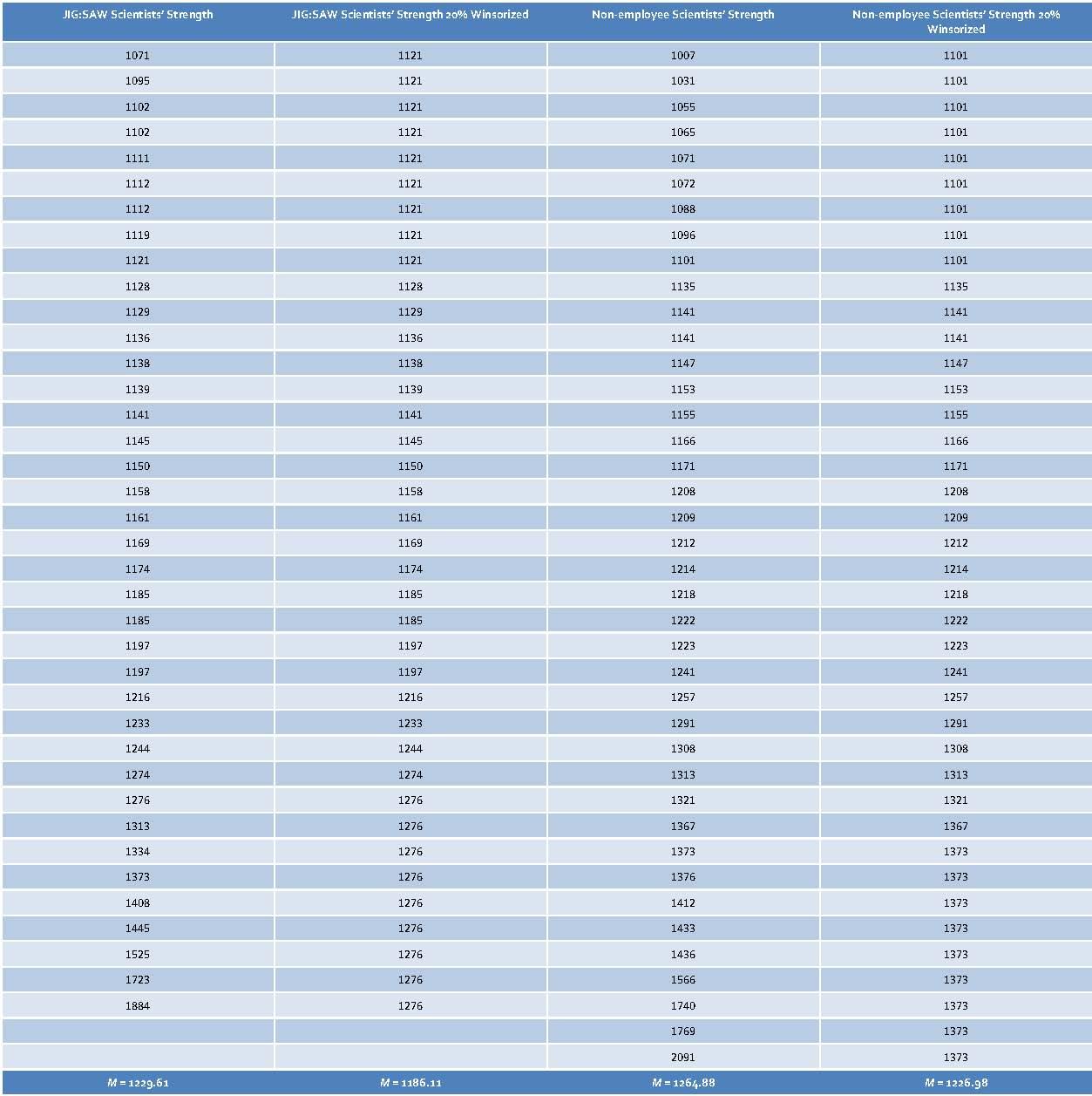
To calculate the 20% winsorized mean, we need to replace the top and bottom 20% of scores with the next highest or lowest score. If we start with the JIG:SAW employees, there were 38 in total and 20% of 38 is 7.6, but we would round this up to 8 because we need a whole number. Therefore, we take 8 scores from each end of the distribution and replace them with the next highest or lowest score. First, I put the scores into ascending order. I have done this in Table 3 (first column). In the second column, I have replaced the largest 8 scores with the next largest score (1276), and replaced the lowest 8 scores with the next lowest score (1121). To get the 20% winsorized mean, calculate the mean of the second column:

I did exactly the same for the non-employees: because there were 40 scores in total and 20% of 40 is 8, I took the raw scores (column 3) and replaced the largest 8 scores with the next largest score (1373), and replaced the lowest 8 scores with the next lowest score (1101) — see Table 3 (final column). To get the 20% winsorized mean, calculate the mean of the final column:

Table 3: Raw data and 20% winsorized data for the JIG:SAW and non-JIG:SAW scientists’ strength scores

If we collate our answers from the previous puzzles it will make it easier to compare the robust estimates (Table 4). Looking at the means based on the raw scores, we can see that there is not much difference between the mean strength of scientists in the JIG:SAW and non-employee groups; the non-employees were slightly stronger than the JIG:SAW employees, but not by very much. Looking at the 20% trimmed and 20% winsorized means, these robust estimates are smaller than the raw mean by about 40–45 units in the non-employee group, and smaller by about 40–50 units in the JIG:SAW group. In other words, the change in the mean is fairly similar in the two groups, and the differences between the groups have stayed fairly similar (raw mean difference = 35.27, trimmed mean difference = 43.2, winsorized mean difference = 40.67). (You might think that 35.27 is quite different to 43.2, and you’d be correct if the scale of measurement perhaps ranged from 0 to 50, but the strength scores range from 1000 to 2000, and in that context a difference of around 8 is not particularly startling.)

Table 4: Various measures of the average strength for the JIG:SAW and non-employee scientists

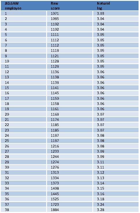
To log transform the JIG:SAW data we need to take the natural log of each score. You can use software such as Excel, SPSS or R to do this for you. I used Excel and pasted the scores into the table.

Table 5: JIG:SAW scientist’s raw scores and log-transformed scores

Bootstrapping is a technique from which the sampling distribution of a statistic is estimated by taking repeated samples (with replacement) from the data set (in effect, treating the data as a population from which smaller samples are taken). The statistic of interest (e.g., the mean, or b coefficient) is calculated for each sample, from which the sampling distribution of the statistic is estimated. The standard error of the statistic is estimated as the standard deviation of the sampling distribution created from the bootstrap samples. From this process, confidence intervals and significance tests can be computed too.