Step	Task	Chapters
1	Think about variables	2
2	Define measures for variables	3
3	Build hypotheses	4
4	Effect sizes, graphs and uncertainty	4–5
5	Identify statistical tests – which and how to report	7
6	Analyse some raw data	7 plus online data generator
7	Consider Type I and II errors	8–10
8	Design experiments	10
9	Plan using more IVs	11–12
10	Analyse some raw data	13 plus online data generator
11	Write the results up	15
12	Plan a follow-up study	1–15

Think about variables

This requires Chapter 2.

We want you to look around your educational setting (e.g. your class group, or people on your degree programme) and see if you can find some example variables.

Our prompts in this table will help you find variables that could be rather interesting. In each case we’ve given you one example to get you started.

Prompt	Write down your variable name here	Write down some possible values here
When students are learning, what types of outcome matter most to them? Give 3 examples	Grades	40, 60, 75
What distinguishes good students from poor students?	Hours studied	0 (no hours extra) 25 (25 hours extra)
What feelings and emotions might students have while they are learning?	Surprise	0 (no surprise at anything) 0.2 (slightly surprised) 1 (amazed)
What sort of activities are available to support learning?	Tutorial attendance	Yes No
Can you think of ways in which students vary that shouldn’t matter for their learning, but that possibly do?	Declared disability	None Physical Mental

Define measures for variables

This requires material from Chapter 3.

In Step 1, you thought up some variables. Now we want you to think in more detail about how you would set these variables up:

• What name should each one have? Keep names short and easy to understand.
• What type will your variables be? Interval or Categorical?
• What range of values will your variables have? For Interval variables, remember that 96% of all participants lie within the range +/– 2SD.

Look back at your variables, then complete the following table. Feel free to change your variables if you have better ideas now. As before we have given you one example to get started.

Prompt	Variable name	Variable type	Variable values – mean and SD (interval) or categories (categorical)
When students are learning, what types of outcome matter most to them? Give 3 examples	Grades	Interval	mean = 60, SD = 10
What distinguishes good students from poor students?	EngagementHours	Interval	mean = 5, SD = 2
What feelings and emotions might students have while they are learning?	Surprise	Interval	mean = 0.2, SD = 0.05
What sort of activities are available to support learning?	Tutorial attendance	Categorical	yes, no
Can you think of ways in which students vary that shouldn’t matter for their learning, but that possibly do?	Declared disability	Categorical	none, physical, mental

Build hypotheses

This requires material from Chapter 4.

Now we will use the variables you have developed in Step 1 to build a few hypotheses. Remember that a good hypothesis is one where the result is unknown and potentially interesting.

We ask you to consider for each of your hypotheses how informative and interesting the results will be:

• Hypothesis – use this notation IV → DV
• Informative – a result will be informative if it tells us something we didn’t know before.
• Interesting – a result is interesting if it leads to new questions.

Look back at your variables from Steps 1 and 2, then complete the following table. As before we have given you one example to get started.

Prompt	Hypothesis	Informative	Interesting
DV: choose a variable from learning outcomes IV: choose a variable from good vs poor students	Engagement → Grades	Slightly (it is obvious)	No
DV: choose a variable from feelings & emotions IV: choose a variable from learning activities
DV: choose a variable from learning outcomes IV: choose a variable from feelings and emotions
DV: choose a variable from learning activities IV: choose a variable from shouldn’t matter
Freestyle: make a hypothesis with any of the variables

Think about effect sizes, graphs and uncertainty

This requires material from Chapters 4 and 5.

Now we will examine these hypotheses. What effect size do you expect it will have? Can you visualize what the graph showing the effect might look like?

• Hypothesis – use this notation IV → DV
• Predicted effect size – choose from small medium or large. Can you say whether this is likely to be a positive or negative effect?
• Graph – in Chapter 4 you will have seen graphs of the relationships between variables, depending on variable type. Looking back to Step 3, choose the right graph providing the types of your variables. Use the graph to show both (i) the effect you expect to see and (ii) the uncertainty you expect.

→ This bit can work several ways: download and open this document in Word and paste in a graph that you make up in Excel; or print out this activity and fill it all in by hand

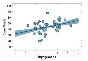
Uncertainty is shown in graphs as either error bars (for line graphs and bar charts) or as the shaded area around a regression line (as in the example below). You can draw these in for yourself, but do think carefully about what they mean.

Look back at your hypotheses from the previous table, then complete the following table. As before, we have given you one example to get started.

Prompt	Predicted effect size	Predicted graph of effect
Hypothesis 1: choose one from the previous step	Engagement → Grades small, positive
Hypothesis 2
Hypothesis 3

Identify statistical tests

This requires material from Chapter 7.

Now we will examine the hypotheses you have been developing. This time we are asking a very simple question about the null hypothesis test.

• Hypothesis – use this notation IV → DV
• Test name – choose one from Chapter 7
• Test statistic – usually this is a single letter (t, r, F, chi²).
• Sample size – just choose a number, make it bigger if the effect size is expected to be small
• APA format – write this with an invented value for the test statistic and p-value

Look back at the previous steps, then complete the following table. As before we have given you one example to get started. Try picking hypotheses that lead to different statistical tests instead of repeating yourself.

Prompt	Test name	Test statistic	Sample size	APA format
Hypothesis 1: choose one from the previous step	Engagement → Grades Pearson correlation	r	42	r(40) = 0.2, p = .08
Hypothesis 2
Hypothesis 3

Analyse some raw data

This requires material from Chapter 7 and you will use the online data generator to make the data.

In this step, we are going to create some data for your hypotheses from Step 5 and see what the data has to say. The book’s website has a simple data generator. It is an MS Excel™ file with two important sheets: when you download it, give it some time to load. The first sheet (called the Design Sheet) is where you enter the details of your hypothesis, variables and expected effect sizes. When you have finished doing this, you will find that there is a second sheet that now contains data. This data is not real, but it does conform exactly to your hypothesis specifications. You task is to use this data file to produce real graphs and APA statements for this data; analyse the data using the software of your choice to conduct the tests that you listed in Step 5. Just like in real research, the data you get is always different from anyone else’s and different every time you do it. If you wished, you could see for yourself how sampling error works.

Look back at Step 5, then analyse your data and complete the following table. As before, we have given you one example to get started.

Prompt	APA format statement	Graph of result
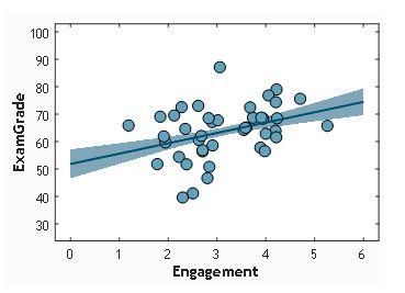
Hypothesis 1: choose one from the previous step	Engagement → Grades r(40) = 0.2, p = .08
Hypothesis 2
Hypothesis 3

Consider Type I and II errors

This requires material from Chapters 8 to 10.

Before we start a study we can have a precise idea of what the probability is that we will make a Type I error, and a vague idea about the probability that we will make a Type II error.

We will leave you to get the probability of a Type I error, just saying that we will be applying the conventional alpha value of 0.05.

For the probability of a Type II error, we will give you a bit of guidance with this table. It shows for various combinations of population effect size and sample size, what the probability of a Type II error would be.

	Small effect (r = 0.1)	Medium effect (r = 0.2)	Large effect (r = 0.4)
n = 20	92%	85%	53%
n = 40	90%	75%	24%
n = 80	85%	55%	3%
n = 160	75%	27%	1%

You must judge what population effect size you should consider using.

Look back at your hypotheses from the previous table, then complete the following table. As before we have given you one example to get started. Our example falls close to the n = 40 row of the above table, and is somewhere between a medium and large effect size, hence our estimation of a 40% probability.

Prompt	Population effect size	Sample size	Probability of a Type I error	Probability of a Type II error
Hypothesis 1	Engagement → Grades 0.33	42	5%	40%
Hypothesis 2
Hypothesis 3

Design experiments

This requires material from Chapter 10: the focus is on between vs within experiments.

Here, we have designed an example experiment. In our example experiment, we are going to compare two different interventions we could apply to participants to see whether they change the DV of our choice. This time we are asking for the following details:

• DV – go back to Step 3 to look at which variables you chose to be DVs in your hypotheses
• Interventions – describe two
• Design – between or within
• Graph of effect – as we did in Step 2

Instead of picking DVs from your current list, you will probably need to think of new ones, which revolve around the idea of an intervention. It is your choice whether the intervention requires between or within groups of participants. You are also not restricted to only two categories.

Prompt	Intervention groups	Between/within	Graph of effect
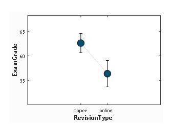
DV: create new ones, or modify some DVs that you already have	DV = Grades Revision with online material Revision with printed material	Between
DV 2:
DV 3:

Plan using more IVs

This uses materials from Chapters 11 to 12.

Of course, many studies do not just investigate one IV. Think about how different variables that you have considered during this series of steps could come together to form interesting hypotheses with two IVs and one DV. Fill out the following table with some examples. If you want, you can add in new ideas instead of using variables you have already written down.

• Hypothesis – use this notation IV1 + IV2 → DV
• Interaction – do you expect an interaction? Remember that an interaction is like a switch. In our example, we think that the effect of engagement of grades doesn’t depend on whether you are anxious or not
• Covariation – do you expect covariation? In our example, we think that the more anxious you are, the less you will engage.

Prompt	Hypothesis	Interaction	Covariation
Hypothesis 1: choose one from the previous step	Engagement + Anxiety → Grades	No	Yes
Hypothesis 2
Hypothesis 3

Did you understand the difference between an interaction and covariation?

• In an interaction, how much one IV affects the DV depends on the other IV. In our example, engagement is always good for you, regardless of whether you are not anxious or very anxious. So there is no interaction.
• In a covariation, the two IVs affect each other as well the DV. Engaging always gives you higher grades. Being anxious always gives you lower grades (this isn’t true actually but it is our example). But on top of that, being anxious possibly means you will engage less: the two IVs are related.

Analyse some raw data

This requires material from Chapter 13 and the online data generator.

In this step, we are going to create some data for your latest hypotheses with more than one IV and see what the data has to say. You should have experienced the data generator as part of Step 6; you can use the same MS Excel™ file for this piece of work. However, try adding in one or two new variables to keep practising your research design skills.

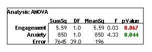
Recall that the file has a Design Sheet and a Data Sheet. Once you have a completed Data Sheet (remember, it responds to your Design Sheet decisions), you can import this data into your software of choice. First analyse the data with a General Linear Model, and then by using an ANOVA. All we are asking is for you to fill in the table of outputs. Remember that in Chapter 13, we highlight the difference in how these two test styles work.

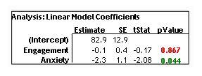
For the General Linear Model, you should use software available to you to obtain a table of the coefficients, their standard errors, t-statistics and p-values.

For the ANOVA, produce the equivalent table of SumSQ, MeanSQ, F-statistics and p-values.

Prompt	General Linear Model	ANOVA
Hypothesis 1	Engagement + Anxiety → Grades
Hypothesis 2
Hypothesis 3

Write the results up

This requires material from our closing chapter, ‘Finishing with One Bigger Picture’, and previous chapters.

There is no point in doing research and then not telling others about it. The write-up is important so that your participants can feel that the time they gave you was worthwhile. Before the specifics, we have a most important thing to say.

Be honest with your write up. Honestly. Honesty is the best policy. Let’s have the results you got. Here’s a big one: never be tempted to meddle with the data. And a small one: if you are doing null hypothesis testing, then don’t pretend that p = 0.06 is ‘nearly significant’. If you have agreed to abide by the rules of null hypothesis testing, then do so: you either eject the null hypothesis or you fail to do so.

There is a lot of illusory pressure to find p < 0.05. For a dissertation or other student project, a failure to reject the null hypothesis is maybe the better outcome – the discussion section of the report has plenty to talk about (such as how you would do things differently next time). If you get a significant result, the discussion section hasn’t much to say apart from a general smugness.

It is sensible to distinguish between exploratory research and confirmatory research. Fill in this table based on some of the earlier analyses that you have carried out. Make Hypothesis 3 one of your three-variable (2 IV + 1 DV) hypotheses.

Prompt	APA Statement	Description of result
Hypothesis 1	Engagement → Grades r(40) = 0.41, p = 0.007	A statistically significant relation was found between student engagement and exam grades. The effect size was 0.4, large for Psychology.
Hypothesis 2
Hypothesis 3

Plan a follow-up study

This requires material from the whole book.

In this step, you are going to be creative and think about what studies you should plan next. For this last step, you don’t need any prompts from us – it’s your time to take over. Just write your ideas down below and see what flows. Remember to be creative!