Analyzing Social Networks
Chapter 11: Subgroups
11.10 Problems and Exercises
› Click here to download corresponding data
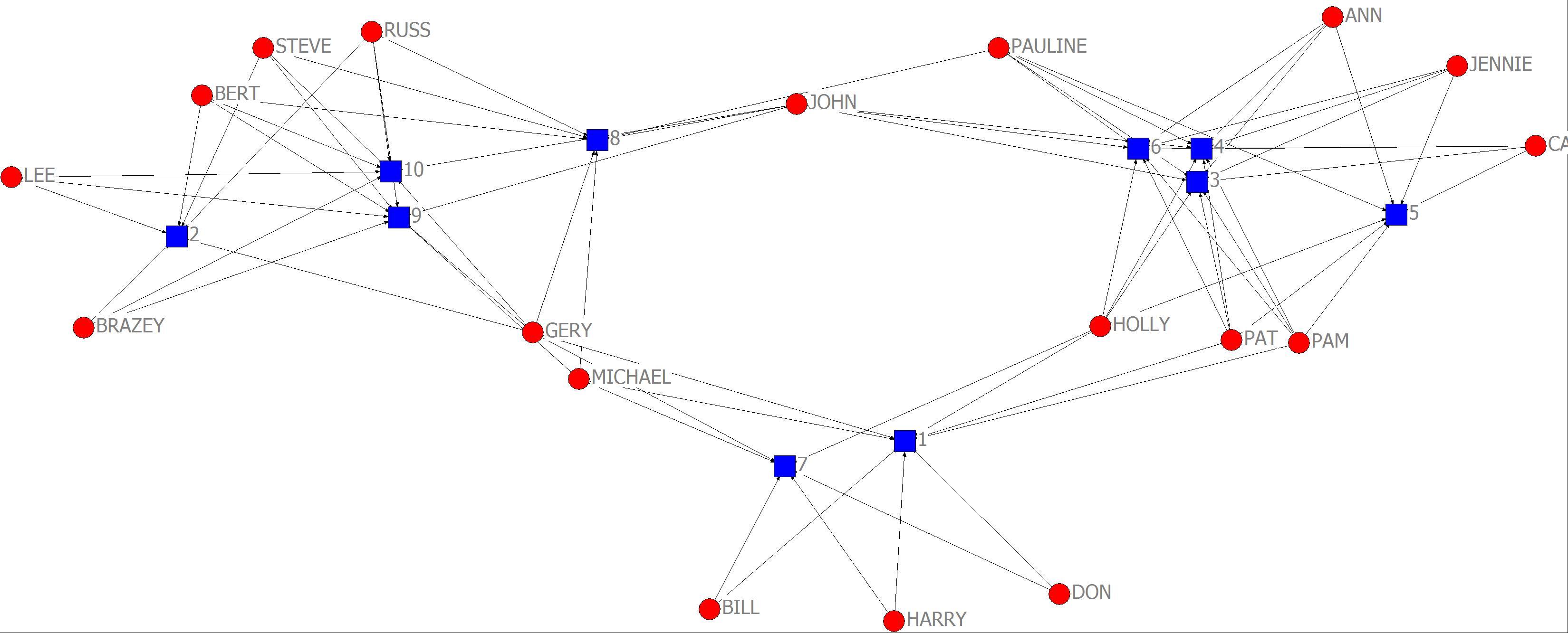
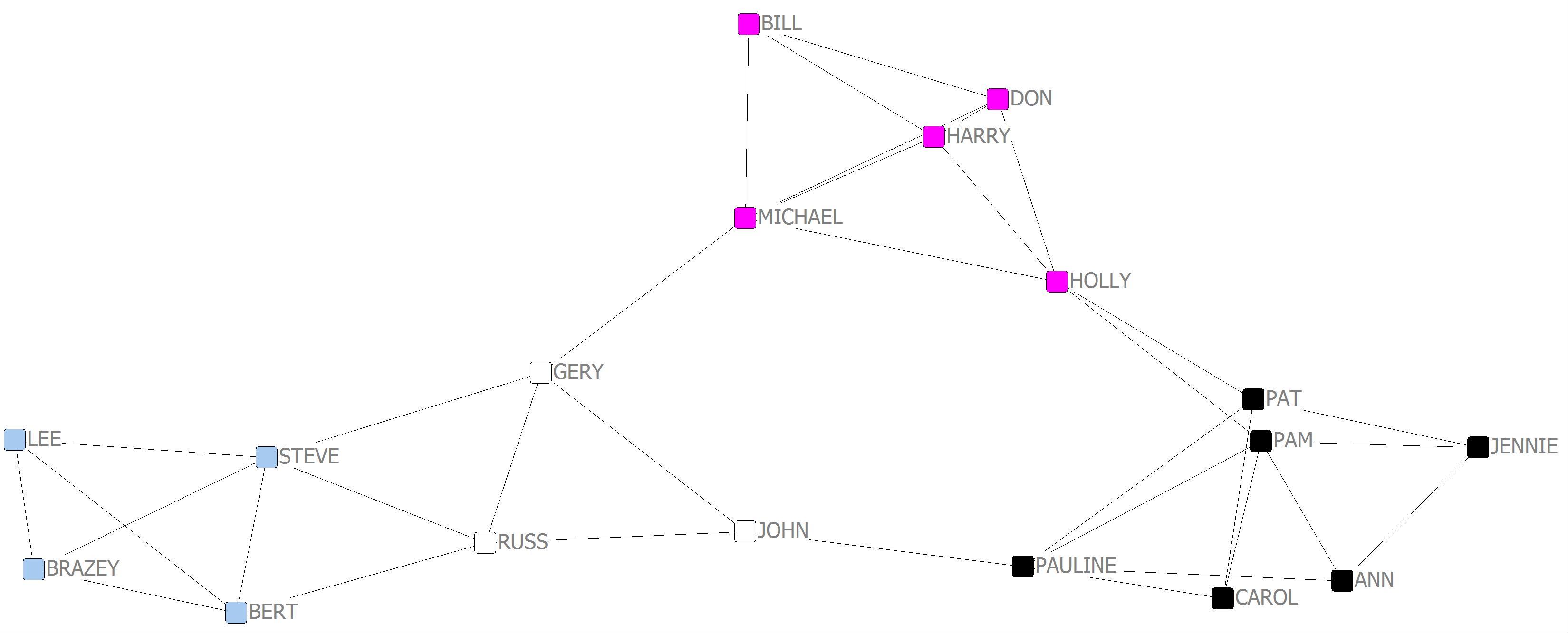
1. The network data in the file “campnet.##h” will be used for the problems and exercises in this chapter. First, we want to symmetrize the network. In UCINET go to Transform|Symmetrize… and input Campnet.##h. In this case symmetrize by using the “Maximum”. Once maximum has been selected click OK. The symmetrized network we will be using is called “campnet-maxsym.##h”. Now visualize the network using NetDraw (this is something you should be able to do by now). With just a visual inspection of the network how might you characterize the subgroupings among actors in the network? Now we want to analyze the network using the various approaches discussed in the chapter for detecting cohesive subgroups.
Campnet network

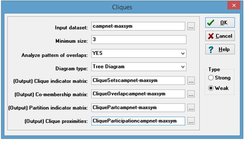
2. Initially we want to identify the cliques in the network. In UCINET go to Network|Subgroup|Cliques… and input the file “campnet-maxsym.##h”. Be sure to name all the output files accordingly. For example, you might want to add the name of the network to the output file default name as in “CliqueOverlapcampnet-maxsym”. Once the file has been loaded and the output files properly named click OK. Be sure to save the “ucinetlog” for later use. How many cliques are there? Are actors members of more than one clique?
There are a total of 10 cliques or maximally complete subgraphs. Yes, there are a number of overlapping memberships in the various cliques. For example, Bill, Harry and Don all share overlapping membership in cliques 1 and 7.
Running Cliques
Clique membership

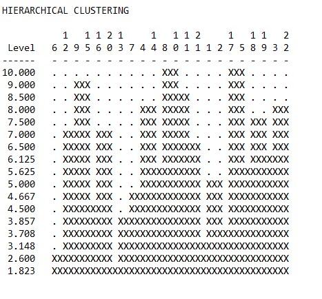
3. Using the same output from Problem 2 above, what does the “Actor-by-Actor Clique Co-Membership Matrix” tell you? Using the “HIERARCHICAL CLUSTERING OF OVERLAP MATRIX” in the same output, how many subgroups would you say are in this network?
Depending on what level one uses to determine the cluster membership, from a simple visual inspection there are clearly three or four obvious clusters. This will be examined more closely in the following exercises.
Hierarchical clustering of overlap matrix

4. We can also examine the actors and the cliques simultaneously. Referred to as the bimodal method, we want to use one of the output files created during the run of the clique analysis in Problem 2 above. This involves the clique participation matrix, which if using the naming method outlined above would be named “CliqueParticipationcampnet-maxsym.##h”. Go to NetDraw and click on File|Open|2_Mode network. Enter the clique participation network and click OK. What does this bimodal representation inform us about the subgroupings in the network?
Similar to the analysis of the overlap matrix, this shows three clear clusters with a possible fourth.
Graph using bimodal method
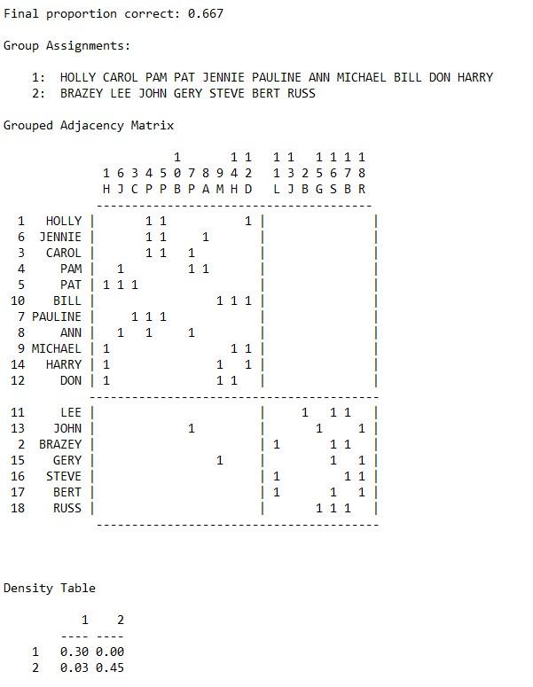
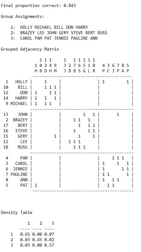
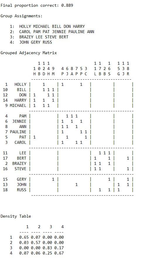
5. Another way to determine cohesive subgroups is factions. Using “campnet-maxsym.##h” in UCINET go to Network|Subgroup|Factions and load the network. You have to determine the prescribed number of partitions or subgroups in advance. For the purposes of this problem we will run a series of analyses with different numbers of prescribed blocks or subgroups. With number of blocks designated as 2 click on OK. Save the ucinetlog file for later comparison (be sure to save the file to your working folder). Now run the factions again only this time designating the number of blocks as 3 (remembering to save the ucinetlog output). Finally, run the factions again only this time designating the number of blocks as 4 (remembering to save the ucinetlog output). Does a 2, 3 or 4 block solution best reflect the cohesive subgroup structure of the network?
The four faction solution seems to work best. Notice as we move from the two to the four faction solution the final proportion correct increases. Also, notice that the within block densities in the density table are highest for the four faction solution.
Two Factions
Three Factions
Four Factions
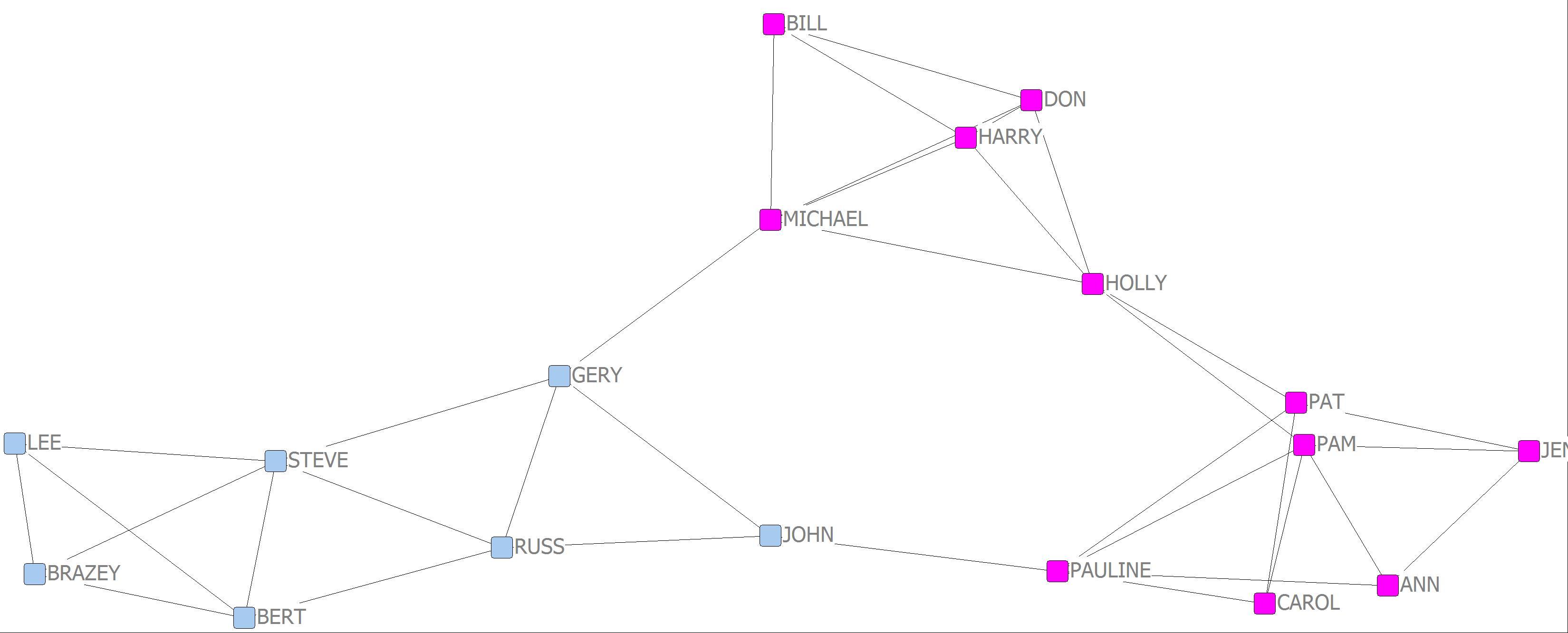
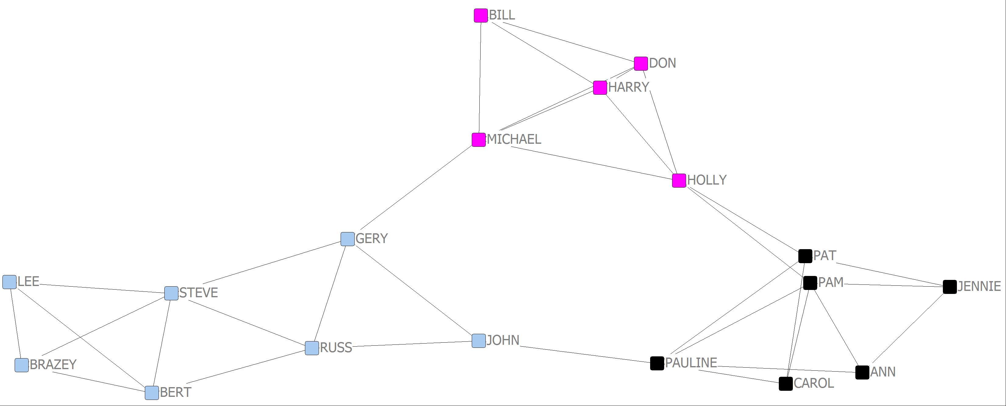
6. Another method for detecting cohesive subgroups, also referred to as community detection, is the Girvan-Newman algorithm. Using the Campnet symmetrized network go to UCINET and click on Network|Subgroup|Girvan-Newman and load “campnet-maxsym.##h” and click OK. The output shows partitioning of the network into subgroups at different levels. However, we can visualize the various levels of partitioning using NetDraw. An output file was produced called “campnet-maxsym-gn.##h”. Go to NetDraw and click on File|Open|Ucinet dataset|Network and enter the Campnet symmetrized network and click OK. We now want to use the Girvan-Newman attribute file containing the partitions. Go to File|Open|Ucinet dataset|Attribute data and load the file “campnet-maxsym-gn.##h” and click OK. The attribute file is now loaded. Now go to Properties|Nodes|Symbols|Color|Attribute-based. Click on the Select Attribute pull down menu. There will be a list of attributes for various levels of partitioning and an attribute for ID. We are interested in the partitions designated with a “C”. So C2 is for two subgroups, C3 for three subgroups and so on. In the pull-down menu click on C2. Two boxes with colors should be displayed representing each of the two partitions. Click on the green check mark. Now go back to the pull-down menu and click on C3 and click the green arrow. Repeat for C4. How do the various levels of partitioning compare?
This yields very similar results to the analysis of overlapping clique membership and of network factions.
Girvan-Newman 2 cluster
Girvan-Newman 3 cluster
Girvan-Newman 4 cluster
8. Cohesive subgroup can also be determined in valued networks. We will use a valued network for the South Pole crew at the end of the winter. The valued network is named “End_Winter_Valued.##h”. Similar to Chapter 6, Problem 4 we can determine cohesive subgroups in this valued network using Hierarchical Clustering. In UCINET go to Tools|Cluster Analysis|Hierarchical and input the name of the network data file. Since this is valued data on a 11 point Likert Scale, with 0 being no social interaction and 10 being a lot, we want to make sure “Similarities” is entered. We will use the default method of WTD_AVERAGE. Also, make sure the “Output Partition Matrix” is properly named for later visualization of the partitions in the network. Once the file is loaded click OK. How many cohesive subgroups would you say are in this valued network?
There are clearly three primary clusters in the hierarchical clustering analysis. Whereas 6 is an isolate, 12, 9, 15, 16, and 20 form a well-organized cluster. These were the science contingent at the station. Two other clusters reflect people who hung out in the bar and those who hung out in the biomed facility.
Cluster Analysis of Valued Relations