Analyzing Social Networks
Chapter 12: Equivalence
12.10 Problems and Exercises
› Click here to download corresponding data
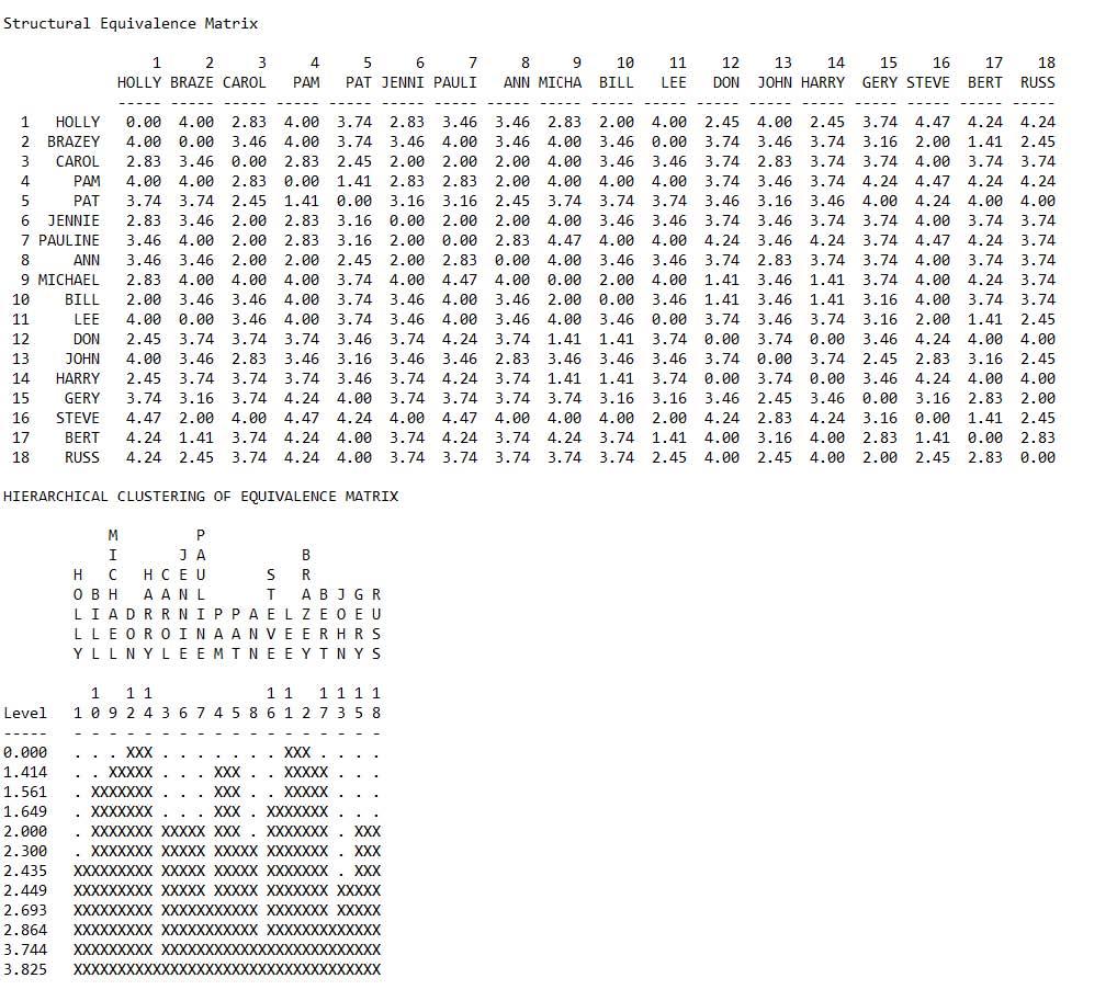
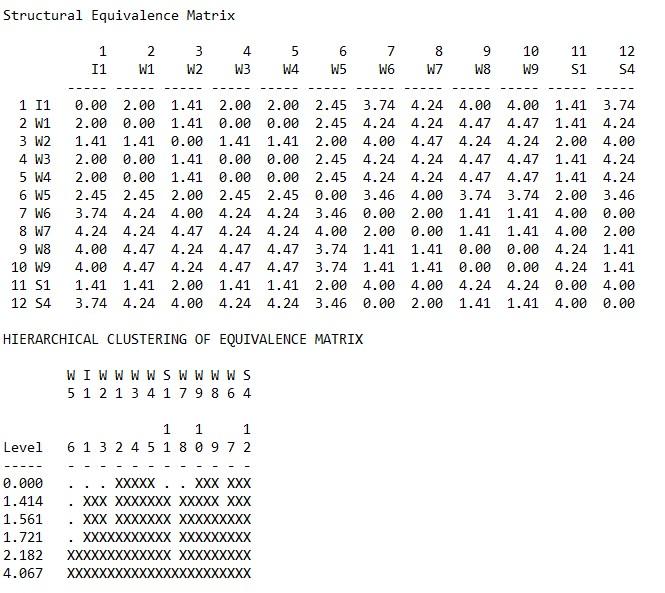
1. Another way to find clusters of nodes in a network, besides cohesion, is by looking at the structural similarity or structural equivalence among nodes. Using the “campnet-maxsym.##h” in UCINET go to Network|Roles & Positions|Structural|Profile… and load the symmetrized Campnet network. Since this is a symmetric matrix we do not need to include the transpose. For the similarity measure use the default Euclidean Distance. Be sure to properly name the output files for future use. For example, they could be named SEcampnet and SEPartcampnet respectively. Once the file is loaded click OK. A ucinetlog file will have the equivalence matrix and an HCL of the matrix. In looking at the clusters in the HCL how does this compare to the identification of cohesive subgroups for the Campnet data in Chapter 11?
There are some similarities. However, Holly and John are connected to clusters at lower levels since their network positions are somewhat unique. Lee and Brazey and Don and Harry are structurally very similar.
Structural equivalence results
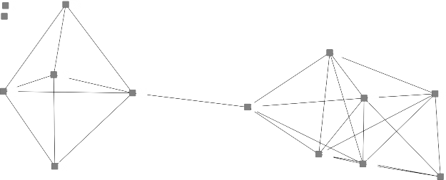
2. Now let’s examine some different ways of looking at measuring the structural equivalence among actors. We will be using the wiring bank room game network called RDGAM.##h. Before running the analysis visualize the network in NetDraw. How many isolates are there? Using this network run a profile similarity analysis as in Problem 1. In UCINET go to Network|Roles & Positions|Structural|Profile… and load the game network. For the similarity measure use the default Euclidean Distance. Be sure to properly name the output files for future use as in Problem 1 above. Click OK. What do you notice about the Euclidean distance between I3 and S2? The two nodes are structurally equivalent in that each is similar in that they are not connected to any nodes in the network. We should remove the isolates and run the analysis again. To remove the isolates, go to Data|Remove|Remove isolates. Enter the games network and click OK. Note that the output file is automatically named RDGAM-NoIsolates. In UCINET go to Network|Roles & Positions|Structural|Profile… and load the game network with isolates removed. For the similarity measure use the default Euclidean Distance. Be sure to properly name the output files for future use as in Problem 1 above. Click OK. Reviewing the ucinetlog, which actors are structurally equivalent? What is it about actor W5 that makes him/her structurally unique (look at the network visualization of the games network)?
There are two isolates. In the hierarchical clustering the two are seen as structurally identical, that is they are both isolates. Actor W5 is what we would call structurally unique. No other actor in the network is structurally similar to W5.
RDGAM Network
Structural equivalence of RDGAM including isolates
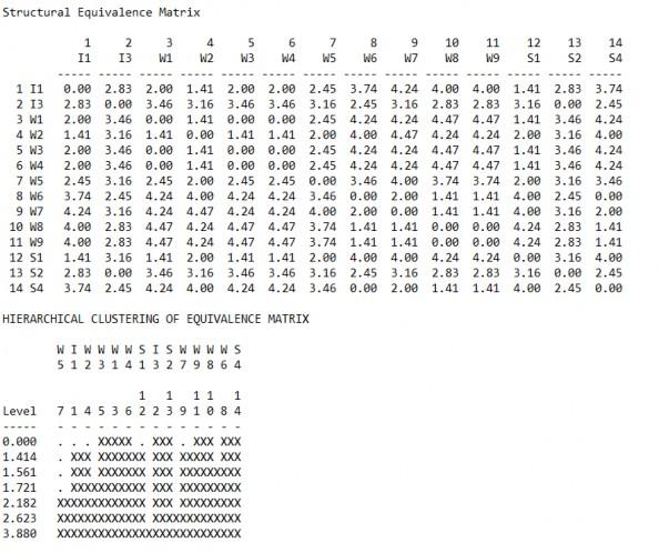
Structural equivalence of RDGAM including isolates removed
RDGAM network with no isolates

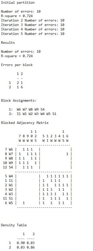
3. Now let’s use the same WIRING games network to fit a blockmodel. In UCINET go to Network|Roles & Positions|Structural|Optimization|Binary and load the RDGAM-NoIsolates network. For this run make the number of blocks 2. Click OK. What can you conclude about the structure of the network?
There are clearly two blocks or partitions in this network. There are extremely high densities of ties within blocks and very few ties between blocks. In fact, there is only one edge connecting the two.
Results
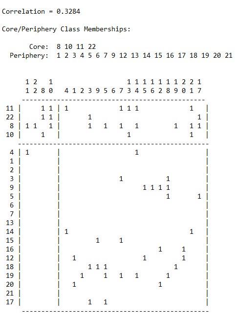
4. In this problem we want to test for core–periphery structures at the beginning and end of the winter for the South Pole networks. Johnson et al. (2003) found that networks that had core–periphery structures tended to have higher group morale. The data involve strong ties among crew in terms of who interacts socially with whom. In UCINET go to Network|Core/Periphery|Continuous and load “Beginning_Winter_Valued_GT_6” and hit OK. Be sure to save the ucinetlog output for later comparison (you can also minimize it for later use). Do the same for the “End_Winter_Valued_GT_6.” Run the analysis again only this time use the categorical model for both time periods. How did the core–periphery nature of the network structure change over the course of the winter?
This is very similar to the analysis of changes in cohesion over time for this network. The beginning of winter had more of a core/periphery structure that did the end of winter. This reflects the evolution of divisions within the network throughout the winter months.
Partial results for beginning of winter continuous
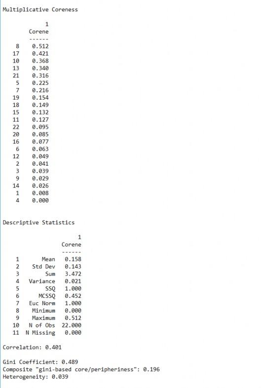
Partial results for end of winter continuous

Partial results for beginning of winter categorical
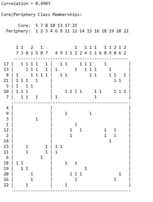
Partial results for end of winter categorical