Analyzing Social Networks
Chapter 13: Analyzing Two-mode Data
13.9 Problems and Exercises
› Click here to download corresponding data
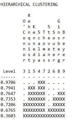
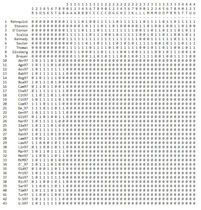
1. For the problems in this chapter we will use the United States Supreme Court decisions in the Rehnquist court (1986–2005) for the year 1997 (SupremeCourt97.##h). The data consist of the nine justices’ decisions on n cases (for matters of simplicity a 1 reflects agreement with the majority decision while a 0 reflects agreement with the minority decision). First visualize the two-mode network using NetDraw. Go to NetDraw, click on the File|Open|Ucinet dataset|2-Mode network and enter the two-mode matrix and click OK. Do there appear to be any patterns with respect to the clustering of the justices? If so, describe the patterns.
There are some Justices clustered more to the right reflecting more and one more spread out to the right. These roughly fall along the lines of conservative justices to the left and more liberal justices to the right.
2-Mode Network of Supreme Court for 1997
2. It is important to visualize the relationship among justices vis-à-vis court decisions on cases and the relationship among court cases vis-à-vis the justices. For this we convert the two-mode matrix into a one-mode matrix of relationships either among cases or justices. The converted one-mode is called an affiliation network.
a. Create an affiliation network of relations among justices. In UCINET go to Data|Affiliations(2-mode to 1-mode) and input the Supreme Court two-mode matrix. Since the justices are the rows of the matrix the “Mode:” to the far left should be highlighted as “Rows”. In this example use the default “Method” sums of cross-product (overlaps). Click OK.
Results for affiliation of Justices
c. Create an affiliation network of relations among cases. In UCINET go to Data|Affiliations(2-mode to 1-mode) and input the Supreme Court two-mode matrix. Since the cases are the columns of the matrix the “Mode:” to the far left should be highlighted as “Columns”. In this example use the default “Method” sums of cross-product (overlaps). Click OK.
Results for affiliation of cases
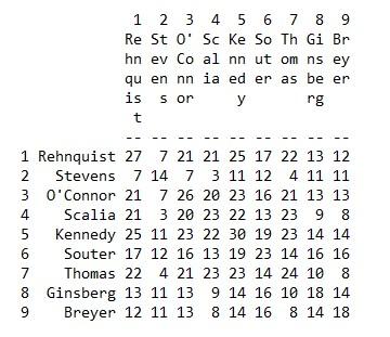
3. Another way to treat two-mode matrices as one-mode data is to convert the matrix to a bipartite network. Using the original two-mode Supreme Court matrix (SupremeCourt97.##h), in UCINET go to Transform|Graph Theoretic|Bipartite… and input the two-mode matrix and then click OK. How would you now characterize the rows and columns of the resulting bipartite matrix?
This is now a one-mode matrix where cell values for any relation between a Justice and a case is 0. The advantage of a bipartite network is the ability to conduct a broader range of analysis using one-mode approaches.
Bipartite network
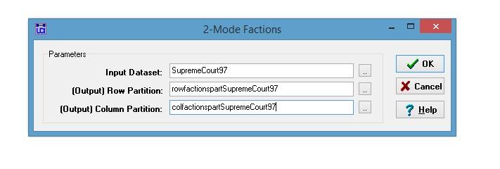
4. The Rehnquist Court was known by the division between liberal and conservative justices. There are a number of ways of looking for cohesive subgroups in the Supreme Court data. We will explore three of them.
a. The first is 2-mode factions. Go to Network|2-Mode networks| 2-Mode Factions and enter the “SupremeCourt97.##h” for input (be sure to properly name the output files) and hit OK. How might you interpret the resulting blocked adjacency matrix in terms of a possible division in the court between liberal and conservative justices?
The blocked adjacency matrix clearly reflect two voting blocks that represent the liberal and conservative split on the court. The density matrix shows strong similarities in decision behaviors within blocks and less similarity between blocks. Many of the 1s in the off diagonal blocks more than likely involve unanimous or near unanimous decisions on cases.
2-Mode Factions Input
Results

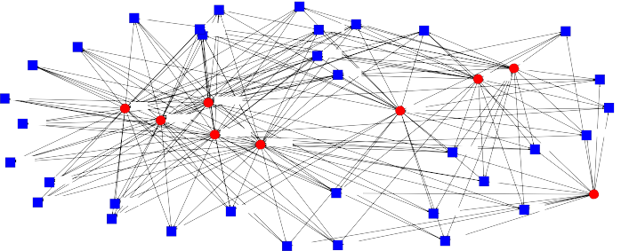
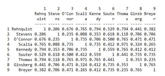
b. As with one-mode networks we can also look for structural equivalence by calculating profile similarities for the rows and columns of the matrix. Since we are mostly interested in the justices we will only examine row profile similarity. In UCINET go to Tools|Similarities & Distances and input the “SupremeCourt97.##h” data file. Make sure that “Rows” are checked. For the purposes of this exercise we will use the “Matches” similarity measure. We will want to use the output file in order to run a cluster analysis (if you input SupremeCourt97 the output dataset will automatically be named SupremeCourt97-Mat-R). This yields a similarity matrix of matches among the justices reflecting similarities in their decision-making behaviors. Which justices have the highest similarity in their decisions across the cases?
Thomas and Scalia are very similar in their decisions on the cases followed by Rehnquist and Kennedy. Among the more liberal Justices, Ginsberg and Breyer are the most similar.
Results for the similarity matrix of matches on court decisions among the justices
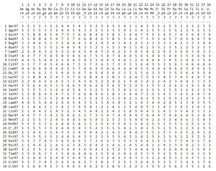
c. The similarity matrix of matches on court decisions among the justices lends itself to hierarchical cluster analysis (HCL) to better understand the presence of subgroupings among the justices. In UCINET go to Tools|Cluster Analysis|Hierarchical… and input the file “SupremeCourt97-Mat-R.##h” and hit OK. What does the cluster diagram tell you about the divisions among the justices?
Similar to the 2-mode factions analysis, the hierarchical clustering shows two primary clusters reflecting a liberal conservative split.
Hierarchical Clustering