Analyzing Social Networks
Chapter 6: Multivariate Techniques Used in Network Analysis
6.6 Problems and Exercises
› Click here to download corresponding data
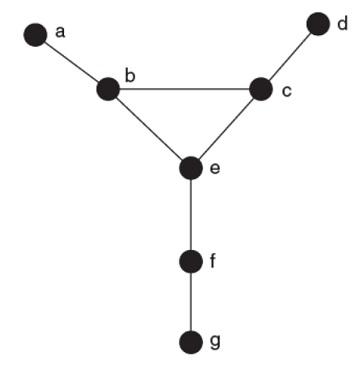
1. Create a UCINET data file for the adjacency matrix for the graph in Chapter 2, Problem 2.
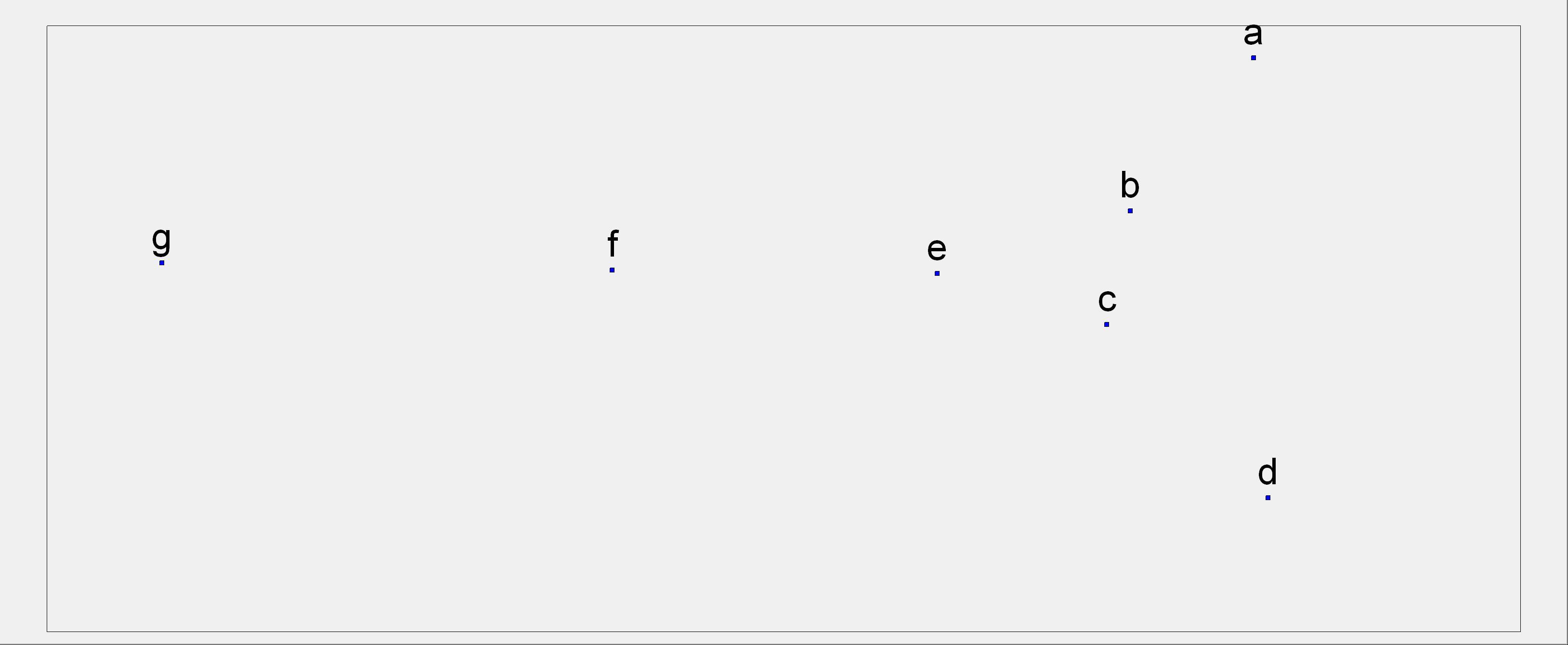
Using UCINET, produce a proximity matrix of geodesic distances (go to Network|Cohesion|Geodesic Distances and upload the adjacency matrix and hit OK). We want to visualize this dissimilarity data using non-metric multidimensional scaling (MDS). To visualize the data using non-metric MDS in UCINET go to Tools|Scaling/Decomposition|Non-Metric MDS and enter the name of the data file (note: make certain the “Similarities and Dissimilarities” is designated properly). Press OK to run. How would you characterize the spatial proximity among the nodes?
This yields a very similar layout of the network (with ties not shown)
MDS Results for the Geodesic Distances from the Network in Chapter 2
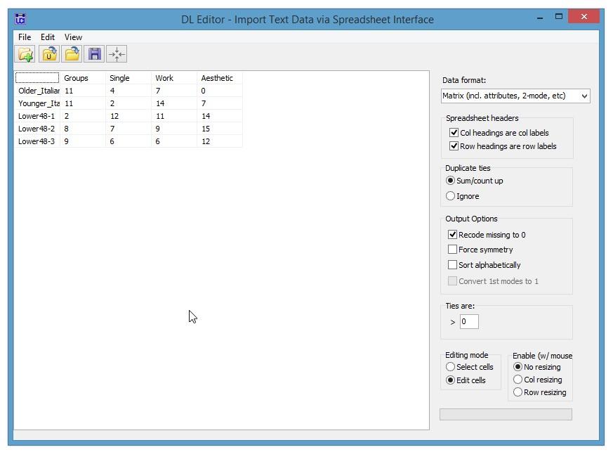
2. The data below came from a study of the social networks of Alaskan salmon fishers in a multi-ethnic fish camp (Johnson and Griffith, 1998). Selected members of the network were given cameras and asked to take pictures of anything that was of interest to them. The resulting pictures were then coded by theme and compared. The table shows the number of photos by each actor involving pictures of groups, pictures of single individuals, pictures of people working, and aesthetic pictures such as animals and sunsets. This table compares the pictures of two Italian fishers with three non-ethnic fishers (Lower48).
- Enter the data in a matrix format in Excel and import the data into UCINET using the DL Editor (in the DL editor open the Excel file and save the file as a UCINET data file using the “Matrix (incl. attributes, 2-mode, etc.)” in the “Data format” menu.) Save the file as “CA_ethnicicty_example”.
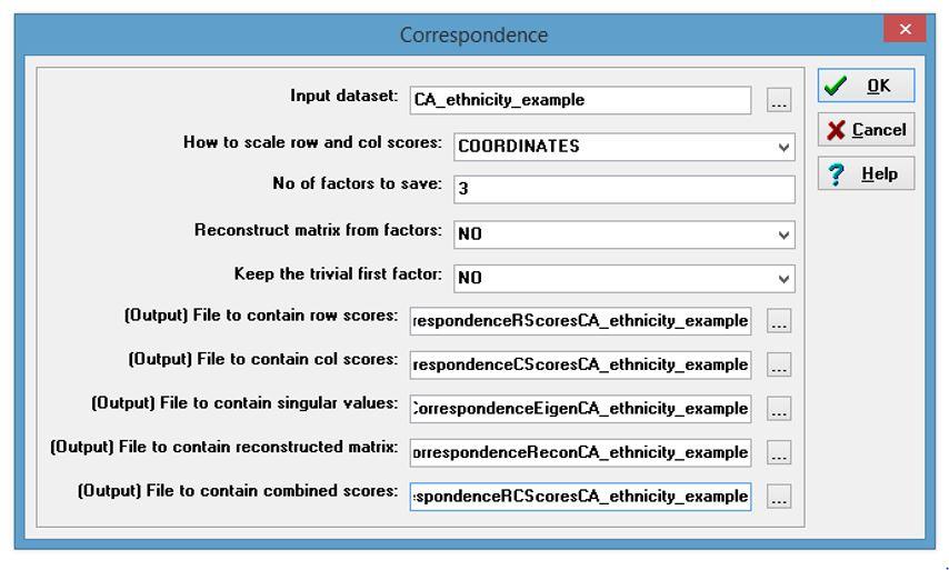
- We want to explore the relationship between ethnicity and the thematic content of pictures. To do this we want to visualize the relationship between and among themes and the ethnicity of the fishers. For this we want to run a correspondence analysis. Under “Tools” in UCINET select Tools|Scaling/Decomposition|Correspondence and enter the name of the data file (CA_ethnicicty_example.##h). Press OK to run.
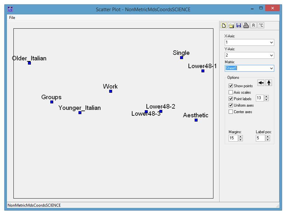
- Based on the correspondence analysis what might you conclude about the differences and similarities in the thematic content of the pictures between Italians and non-Italians?
Data:
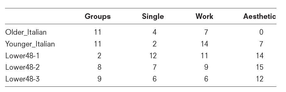
The Italians tended to take more pictures involving multiple individuals (Groups), while the Lower-48 fishers tended to take aesthetic photos such as landscapes and sunsets. However, both took pictures of people working (e.g., fishing, mending nets) reflecting the occupational setting.
Excel file opened in the DL Editor (file saved as a UCINET dataset called CA_ethnicity_example)
Input the example file in Correspondence Analysis
Results of the Correspondence Analysis
3. For this problem we will use the network “Science_Collaboration.##h”. This is a matrix containing the number of grants researchers in a university shared in common as principle investigators, co-principle investigators and/or co-investigators. The number in the cell of the matrix reflects the number of research grants two researchers have in common. We want to visualize these similarity data using non-metric multidimensional scaling (MDS). To visualize the data using non-metric MDS in UCINET go to Tools|Scaling/Decomposition|Non-Metric MDS and enter the name of the data file. Press OK to run.
The Science Collaboration MDS
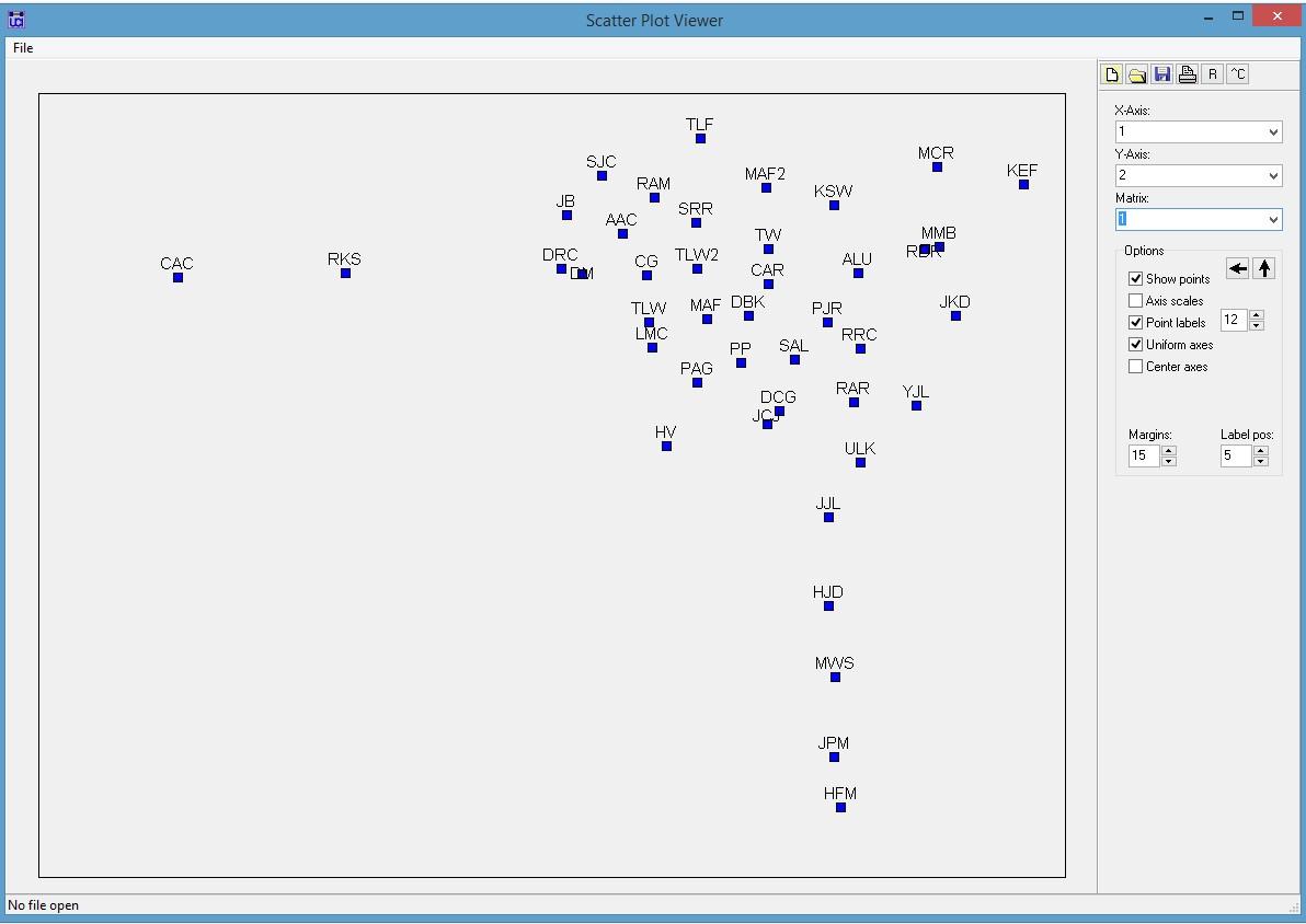
Answer: There is a core set of collaborators with two collaborative chains (DRC->RKS->CAC and JUL->HLD->MWS->JPM->HFM). There is also some clustering in the core from right to left as is evident in the hierarchical clustering. In particular there is a highly overlapping cluster of three ecologists to the upper right of the configuration.
MDS Output including Stress
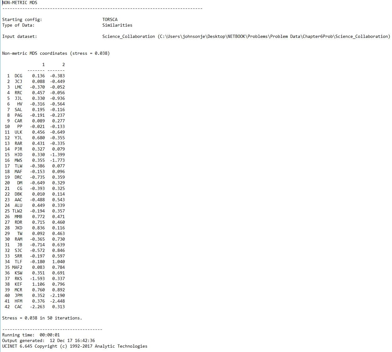
Answer: Stress is a measure of distortion in an MDS map. In metric MDS, stress is evaluated on the basis of a linear relationship between the input proximities and the resulting map distances, very much like the least squares criterion of ordinary regression. As a rule of thumb, we consider stress values of less than 0.2 to be acceptable when using metric MDS. In non-metric MDS, stress is evaluated based on a monotonic (ordinal) relationship such that stress is zero if the rank order of input proximities matches the rank order of map distances. By convention, we consider stress values of less than 0.12 acceptable for non-metric scaling. In this case, the stress value in two dimensions is 0.038 which is very good.
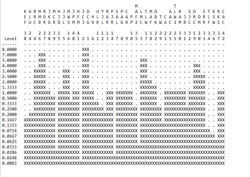
4. For the same proximity matrix used in the MDS example above, run a hierarchical cluster analysis (HCL). To run the HCL go to Tools|Cluster Analysis|Hierarchical and input the name of the data file (make sure to use “Similarities”). For the purposes of this example use the default method “WTD_AVERAGE (average between all pairs)”. Similar to the MDS example above, how would you characterize the subgroupings of the research collaborations?
There is a strong ecologist’s cluster including KEF, ALU, RRC, MMB, JKD and MCR. The chain at the bottom of the MDS forms a cluster (HJD, JJL, MWS, JPM and HFM). JCJ and DCG, both anthropologists, have the strongest relationship (most number of grants in common) and are in a cluster with some fisheries biologists. The cluster LMC, TLW, MAF and DBK is another cluster of collaborative ecologists. The two at the end are from the chain to the left in the MDS, and the scientists in between, form a cluster primarily made up of geologists (TW through TLF).
Hierarchical Clustering output