Analyzing Social Networks
Chapter 8: Testing Hypotheses
8.10 Problems and Exercises
› Click here to download corresponding data
1. It is sometimes important to hypothesize about the factors that might influence the formation of dyadic ties in social networks. The first problem involves the testing of a dyadic hypothesis. For this problem we will be using the Zachery karate club dataset which has already been unpacked. The two networks are named ZACHE.##h and ZACHC.##h. ZACHE represents the simple presence or absence of ties between members of a Karate Club, and ZACHC contains valued data counting the number of interactions between actors. In UCINET go to Tools|Similarities and Distances and use the cross-product measure to compute similarities among the rows of ZACHE. (The cross product is a very powerful and common matrix operation that, in this case, will count how many friends each pair of actors have in common.) UCINET will name the output “ZACHE-Cro-P”. Now go to Tools|Testing Hypotheses|Dyadic (QAP)|QAP Correlation and browse to include both ZACHC and ZACHE-Cro-P to be correlated and click okay. What do the results mean? How might this reflect the first part of Granovetter’s famous ‘strength of weak ties’ theory, which states that I have stronger ties (ZACHC) with those people with whom I share more friends in common (ZACHE-Cro-P)?
The moderate and significant QAP correlation (r=0.3659) shows there is a relationship between the number of friends actors have in common and the extent to which they interact with one another. This is not surprising, but does reflect the tendency to interact more with actors with whom you share friends. The notion of the ‘strength of weak ties’ is that you get less novel information from your circle of friends since everyone has access to the same information, the information is redundant. It is with weaker ties outside that circle that an actor gains more novel information (e.g., information about jobs).
ZACHE-Cro-R

ZACHC

Loading files for the QAP analysis

Results

2. For testing a monadic hypothesis, we will be using the KRACK-HIGH-TEC data that contain three dichotomous relations (REPORTS_TO, ADVICE, FRIENDSHIP). HIGH-TEC-ATTRIBUTES contains several attributes about the nodes in KRACK-HIGH-TEC, including Age, Level (CEO, Manager, Staff), Tenure, and Department. We are going to use the ADVICE network dataset. In UCINET go to Network|Centrality and Power|Degree and load the ADVICE network, using the directed version (lower left), telling it NOT to treat the data as symmetric. By default, it will name the output “ADVICE-deg”.
Loading the file

The Centrality Results

a. We are particularly interested in who is sought after for advice, which is captured by indegree centrality. So, we are going to pull out just that column from the results, by using Data|Filter/Extract|Submatrix. Specify “ADVICE-deg.##h” as your input dataset and that we want to “Keep” “ALL” rows. Then click on the L to the right of the box for “Which Columns” and select the column labeled “InDeg” (for indegree) and call your output dataset ADVISING. This is a measure of how many people said they sought advice from each person.
Advising file

b. Now display (D) the HIGH-TEC-ATTRIBUTES dataset to determine which columns the AGE and TENURE attributes are in. To do that go to the “D” in the icon menu and click on the attribute file. Now, it is common wisdom that people look to the ‘senior’ people for advice, but is unclear in an organizational context whether senior is ‘older’ or ‘longer tenured’. You will test if either of these is supported by the data. In UCINET go to Tools|Testing Hypotheses|Node-Level|Regression specifying ADVISING for your dependent dataset with the appropriate column (Indeg) and HIGH-TEC-ATTRIBUTES and the appropriate columns for your independent dataset (i.e., first adding age and then adding tenure) and set the number of permutations to 10000. Now click OK. Which meaning of ‘senior’ do the data support? Why did we use the Regression option of Node-Level instead of T-Test or Anova? When would we use those?
In this case, the node variable ‘Tenure’ does best in explaining advising indegree centrality. If we were doing this analysis at the node level using a categorical instead of continuous independent variable, it would then be appropriate to use a T-Test or ANOVA for testing a given hypothesis.
Node Level Regression

Results

3. In this problem, we will test a multivariate dyadic hypothesis using the WIRING dataset. This is a stacked dataset which includes many different files. This is a dichotomous adjacency matrix of 14 employees of the bank wiring room of Western Electric used in the famous Hawthorne Studies. Ties are symmetric and represent participation in games during work breaks. RDGAM records people playing games together, RDCON records conflict between people, RDPOS is positive interactions, RDCON is negative interactions. The dataset has been unpacked. In UCINET go to Tools|Testing Hypotheses|Dyadic (QAP)|QAP Linear Regression|Double Dekker Semi-Partialling MRQAP. Put RDCON (conflict between members about whether the windows should be open or shut) in as the dependent variable. Put in RDPOS (positive relationships), RDNEG (negative relationships), and RDGAM (playing games together) as independent variables. Before running it, what do you think would most significantly predict conflict? After entering the networks click OK. Are your results what you expected? How would you explain the results?
The MRQAP shows that whom one plays games with is significantly correlated with conflict (but not strongly). In this case, most of the intergroup conflict (as determined by the games relation) was due to a single member of the front-of-the-room group who fought with many members of the back-of-the-room group.
Entering variables

Results

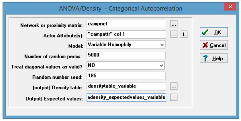
4. For this problem we want to see the extent to which campers’ gender is related to the presence of dyadic ties in a social network of methods training course participants using campnet.##h and campattr.##h. Here we want to test a mixed-dyadic monadic hypothesis. In UCINET go to Tools|Testing Hypotheses |Mixed Dyadic/Nodal|Categorical attributes|Anova Density and run the analysis twice for two different models. For both, specify Campnet as the network matrix, and the “Gender” column of the campattr matrix as the Actor Attribute. For the first run, choose “Constant Homophily” for your model, and for the second, choose “Variable Homophily”. Be sure to save the ucinetlog files for comparison. Interpret both sets of results. Is there homophily? Which gender tends to be more homophilous?
Both methods show slightly higher homophily for the women than for the men. Note the density tables (1=women, 2=men). Also note the regression coefficients in the output for the variable homophily analysis.
Input for constant homophily

Input for variable homophily
Output for constant homophily

Output for variable homophily

5. In this problem, we test a mixed monadic/dyadic hypothesis for the same Campnet network but this time using QAP. In UCINET got to Data|Attribute to matrix, enter the campattr file and create a matrix of exact matches among the actors in Campnet based on Gender. The default name given to the file by UCINET will be “campattr-sameGender”. What does the resulting output matrix show? Now go to Tools|Testing Hypotheses|Dyadic (QAP)|MR-QAP Linear Regression|Double-Dekker Semi-Partialling MRQAP to regress the Campnet network (dependent variable) on this new matrix of gender similarity (independent variable), campattr-sameGender. What do the results show?
Gender has a significant effect on ties within the network suggesting that there is a tendency for the formation of dyadic ties to be influenced by gender. This supports the earlier findings concerning homophily in Problem 4.
Obtaining Attribute Matrix for gender

Gender Matrix

Input for the model

Results
