Short Answer Questions

1. When could we use n rather than (n-1) in the denominator for sample variance? Why?
Main points:

1. When the scores are treated as the population.
2. When μ is known and used in the formula for variance.
3. When μ is known and used in the formula for variance no correction is necessary. The sum-of-squares will not be an underestimate (on average).

2. What is the difference between a frequency histogram and a relative frequency histogram?
Main Points:

1. The units of measurement on the y-axis.
2. For the frequency histogram the units are those as originally measured.
3. For the relative frequency histogram the units are given in either percentage or probability

3. When binning data is required for a histogram, what determines the number of bins?

Main points:

1. Sample size: the smaller the sample size, the fewer the bins, in general.
2. Shape of the distribution: When the shape of the distribution in not normal, often more bins are required.

4. What is the difference between a variance and a sampling distribution?
Main Points:

1. The term “variance” is used to describe the variability of scores about their mean.
2. The term “sampling distribution” is used to described the variability (either empirically or theoretically) of means about their population mean or Grand Mean.

5. What causes variance?
Main Points:

1. Variance exists because people, animals, plants – all members of any class of things – differ.
2. Any variable will be influenced by an unknown number of other variables.
3. Some of these will have a positive effect and some will have a negative effect.
4. Those subjects with more positive effects than negative effects will be above the average performance and those with more negative effects will be below the average performance.
5. The greater the preponderance of positive effects the further above average the subject’s performance.
6. There is a host of influences of which the researcher will be unaware.

6. What does it mean to say a statistic is resistant?
Main Point:

1. Resistant means that single extreme score (or a small number of extreme scores) cannot influence the statistic in question.
2. A sample’s mean and variance are not resistant, although they are unbiased.

7. What does it mean to say a statistic is unbiased?
Main Points:

1.  An unbiased estimator is a statistic whose expected value (E) is the true population parameter.
2. An E is a type of mean. It is a mean of a statistic rather than a mean of individual observations.
3. Furthermore, it is the mean of an infinite number of instances of a statistic or of all possible instances of a statistic.
4. The sample size for these instances must be held constant.

8. When will a single new observation added to a data set leave the mean unchanged?
Main Point:

1. When the single new observation is equal to the original mean.

9. What is the primary difference between parametric and non-parametric statistics?
Main Points:

1. Parametric statistics are based on estimating population parameters such as means and variances.
2. Parametric statistics required certain distributional assumptions such as normality.
3. Non-parametric statistics do estimate population parameters such as the mean and variance.
4. Non-parametric statistics do not require the assumption of normality.

10. Why is the mean not very informative when a distribution is bimodal?
Main Points:

1. When the distribution is normal or at least unimodal the observations will cluster around a single point.
2. The mean will be a useful indicator of the point around which the observations cluster.
3. When the distribution is bimodal, however, the observations will form two clusters.
4. Neither of the resulting clusters will centre on the mean.
5. Thus, the mean will be a false indicator of where the observations cluster.

Data Questions 

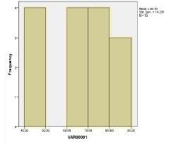
1. With the following data, construct a frequency distribution table and a frequency histogram with bin widths of 10. Observations: 44, 46, 47, 49, 63, 64, 66, 68, 72, 72, 75, 76, 81, 84, 88.

Main Points:

1. Use histogram option, under Legacy Dialogues, under Graphs. Double click on a bar after creating the first histogram. Open the properties window.

 

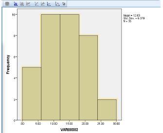
2. With the data below, create a frequency histogram with five categories (bins) on the X axis.
Data: 24, 21, 2, 5, 8, 11, 13, 18, 17, 21, 20, 20, 12, 12, 10, 3, 6, 15, 11, 15, 25, 11, 14, 1, 6, 3, 10, 7, 19, 17, 18, 9, 18, 12, 15.

3. What are the mean, the variance, sampling distribution of the mean, and the standard error of the mean for the data in question #2?
Mean = 12.8286; variance = 40.676; sampling distribution of the mean = 1.1622; standard error of the mean = 1.07804.

4. In terms of the data in question #2, are the skewness and kurtosis values a concern of the researcher who is assuming a normal distribution? (You will need SPSS to answer this question.)
Main Points:

1. According to one rule of thumb, if you divide the statistic (skewness or kurtosis) by its standard error you can evaluate the severity. One rule of thumb is that if the quotient is greater than ±1.96, then the key assumption for parametric tests is called into question.
2. Skewness: -.062/.398 = -.156 (no concern, less than 1.96)
3. Kurtosis: -.778/.778 = -1.0 (no concern, less than 1.96).

5. Create a population of three numbers, e.g. 10, 11, 12. Then analyse ALL possible samples of two, including samples such as 10 and 10. For all samples calculate variance using both n and n-1. Then repeat this analysis using the population mean for each calculation, rather than the individual sample means. In the two series of analyses, which formula (n or n-1) produces an unbiased estimator and why?

1. When the sample means are used to calculate the sample variance (n-1) results in an unbiased estimator.
2. When the population mean is used to calculate the sample variance (n) results in the unbiased estimator.
3. Once the sum-of-squares is no longer underestimated on average (using sample means), then no correction need to be made in the denominator (df).

6. Students are often asked to rate their professor, typically on a 1 to 5 scale: 1 being the lowest ranking and 5 being the highest. In an educational psychology class of 25 students 3 gave their instructor a rating of 1, 4 students gave a rating of 2, 8 students gave a rating of 3, 7 students gave a rating of 4, and 3 students gave a rating of 5.

1. What are the mean and median ratings?
2. What are the variance and standard deviation of the ratings?
3. What might be a problem with computing the statistics in questions “a” and “b”?
4. What are alternative descriptive statistics for those in questions “a” and “b”?

Main points:
Mean = 3.12; median = 3.00
Variance = 1.443; standard deviation = 1.202

• A potential problem is that the ranking may not be on an equal interval scale.
• The alternatives are the mode = 8; the VR = frequency of modal category/ N = 8/25 = .32, the greater the VR the less equally distributed are the observations.

7. A Charity hired three groups of clowns (balloon-twisters, magicians, and jugglers) to perform at a fund raising event. The table shows the number of clowns and the average amount of donations (per clown) raised by the three groups. The jugglers raised a total of $800.

1. How many clowns were there in total?
2. What was the total amount of donations raised by the three groups?
3. How much did the average clown raise?

- 50 clowns in total
- $3700
- $74 

8. Create two distributions with identical means, medians, and ranges. One distribution should be platykurtic and the other leptokuric.
Main Points:

1. Make the means and medians equal, e.g., 10 and 10.
2. Make the two ranges equal, e.g., 5 to 15.
3. Symmetrically cluster one set (equal in number to the first set) of scores between 9 and 11.
4. Symmetrically spread another set of scores between 5 and 15.

9. There are three sections of quiz scores in your class. One has 10 students and a mean of 7. The second has 5 students and a mean of 9. The third has only 5 students and a mean of 5. What is the composite or grand mean of the 20 students?

• 10(7) + 5(9) + 5(5) = 140
• 140/20 = 7 (composite mean)

10. If you took the three means in question #9 (7, 9, and 5) and simply divided by 3 (the number of sections), how would that compare with the composite mean computed in question #9. Why?
Main points:

1. 21/3 = 7
2. Although the sample sizes are unequal, the observations are symmetrically spread around the Grand Mean of 7: five above and 5 below.