Chapter 5: Testing for a Difference: Two Conditons
5.4 Because you know the population mean and standard deviation you may use the standard normal distribution and z to test the difference between the population mean and the sample mean. You also know the critical value of z for a two-tailed test (α = 0.05) is 1.96. You are looking for the sample mean that will result in a z of 1.96. The z-formula now appears differently:
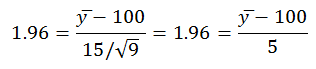
Then solving for y̅ you find
![]()
A mean IQ would need to be 109.8 or greater for you to reject the null hypothesis. This is a two-tailed test and you need to compute how small a mean IQ would need to be to reject the null hypothesis. Thus you need to repeat the calculation using a z of −1.96:
![]()
Thus, the sample mean would need to be equal to or greater than 109.8 or equal to or less than 90.2 for you to reject the null hypothesis with nine students and a population mean and standard deviation of 15 and 100, respectively.
5.9 The easiest way to address the first question is to create two conditions that will have different means. Then distribute the eight scores symmetrically about the two means. Run a t-test. If the test is significant, increase the spread of your scores about their means until the resulting p-value is slightly greater than 0.05. Then increase the greatest score in the condition with the greater of the two means until the t-test results in a p-value less than 0.05. If the original test is non-significant, reduce the spread of your scores about their means until the resulting p-value is only slightly greater than 0.05. Then increase the greatest score in the condition with the greater of the two means until the t-test results in a p-value less than 0.05.
The simplest way to create a data set with an outlier whose presence or absence does not change the outcome of a t-test can depend on whether the t-test without the outlier is significant or non-significant. If the original test is significant, then increasing the greatest score in the condition with the greater mean will not change the outcome. However, an outlier can also change a result from significant to non-significant. This is the case when the outlier is related to the lowest score in the condition with the greater of the two means. The outlier in such cases pulls the two means closer together. You can also produce these results by manipulating the scores in the condition with the smaller of the two means. If the original test is significant, then decreasing the lowest score in the condition with the smaller mean will not change the outcome. When the outlier is related to the highest score in the condition with the lower mean the outlier can change a result from significant to non-significant. The outlier in such cases again pulls the means closer together.
5.12 To begin, to create a data set with two condition means of 20 and 30, distribute their 12 scores symmetrically about those two values. When distributing the score ensure that the row of the highest score in one condition is the same as a row of the highest score in the other condition and that there is a general correspondence in the rank ordering of the scores across the two conditions. The small table below is an abbreviated example of this:
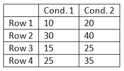
After creating the data set run an independent-samples t-test. (Note: the data will need to be entered differently for the two types of t-tests.) For the independent same t-test the above data would need to be entered as illustrated by the table below:
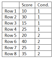
Once the data set is completed run the independent-samples t-test. Adjust the spread of the scores around their means and rerun the test until you produce a result close to but greater than a p-value of 0.05. Once this result is produced transform the data into the format needed for a repeated-measures or paired-samples t-test. Run the paired-samples t-test. It should result in a p-value less than 0.05. This will illustrate how the correspondence in the rows (individual differences) in the repeated-measures (within-subjects) design reduces the variance used to test the difference between the two means. Despite the loss of df, the repeated-measures design almost always produces an increase in statistical power.
The super-challenge question will likely require you to manipulate the data a bit more. The trick is to rearrange the score in one of the two conditions such that there is little to no correspondence between the two rows:

Once the data set is completed run the independent-samples t-test. Convert the data into the form needed for the independent-samples t-test. Adjust the spread of the scores around their means and rerun the test until you produce a result close to but less than a p-value of o.05. Once this significant result is produced transform the data into the format needed for a repeated-measures or paired-samples t-test. Run the paired-samples t-test. It should result in a p-value greater than 0.05. This illustrates how the increased power associated with repeated-measures designs is dependent upon the degree of correspondence between the rows. For example, the subjects who score high in one condition should be the subjects who tend to score high in the other condition.
5.14 The range of the scores in the three dependent variables varies greatly: score1 = 19, score2 = 75, and score3 = 1000. The results of all three independent-sample non-parametric tests (Mann–Whitney) result in the same p-value (0.329). This is produced by the fact that the rank order of the scores across the two conditions is identical in all three variables. Remember, in the non-parametric test the highest score’s relation to the second highest score is the same, regardless of the difference between them, for example, 15 (second highest) and 16 (highest) versus 15 (second highest) and 60 (highest).