Chapter 7: Observational Studies: Two Measurement Variables
7.2 A second assumption is that the observations are independent. The assumption that the observations are independent is not the same as the assumption that the variables are independent. The assumption of the independence of the observations requires that one subject’s response has no effect on another’s response. That is, one subject’s response does not increase or decrease the probability of another subject responding in any particular manner. Furthermore, this assumption requires that there be only one observation per subject. The third assumption is more of an error to be avoided than an assumption. It is the violation of the need to include cases of non-occurrence. We might call this the assumption that all independent observations the researcher collects are included in the analysis. The violation of this assumption most often takes the form of incorrectly reducing a χ2 test of independence to a χ2 test of goodness of fit. Yes, your data satisfy all three assumptions.
7.3 It is simple to change the analysis to an independent-samples t-test. You have a variable, hourcat, which you can treat as the independent variable. You have another variable, quizcat, which you can treat as the dependent variable. You can transform the question into one of the possible randomness of quizcat with respect to hourcat. Your dependent variable might look odd, however, because it has only two possible outcomes, 0 or 1. Such a dependent variable can create problems but let us not concern ourselves with that for the moment. If you run an independent-samples t-test you find the following:
The mean for hourcat (0) is 0.5789 with a standard deviation of 0.50726. In terms of quizcat (1) the mean is 0.1905 and the standard deviation is 0.08781. From the Independent-Samples Test table you will find that the t-value (assuming equal variance) of 2.696 is significant (p = 0.010). This is virtually the same as the p-value from that of the earlier chi-square test (0.011). Because the t-value is significant and the mean of hourcat (1) (above the median number of hours worked) is greater than the mean of hourcat (0), you may conclude that there is evidence that shading the figure results in improved performance.
(If necessary, review the instructions in the previous chapter for running an independent-samples t-test and use quizcat and hourcat as the test variable and grouping variable, respectively.)
7.4 A z-score of 4 means that the corresponding raw score is 4 standard deviations above the sample’s mean. For example, if the mean is 70 and the standard deviation is 5, a score of 90 is 4 standard deviations above its mean [(90 − 70)/5 = 4]. A z-score of 4 indicates the point at which the probability of a score being greater than the observed score (in our current example, a 90) approaches 0.000. (See Appendix A.) The mirror image is the case if the z-score were −4. A z-score of −4 means that the corresponding raw score is 4 standard deviations below the sample’s mean. Again, if the mean is 70 and the standard deviation is 5, a score of 50 is 4 standard deviations below its mean [(50 − 70)/5 = −4]. A z-score of 4 indicates the point at which the probability of a score being less than the observed score (in our current example, a 50) approaches 0.000. (See Appendix Z). Scores with corresponding z-scores of 4 or greater have a disproportional influence on both the mean and the variance. Furthermore, outliers and other extreme scores pull the tail (either the positive or the negative) out away from the mean to such an extent that a skewed distribution is produced.
7.5 Yes, as the number of categories of a discrete variable increases, the more the discrete variable approximates a continuous variable and the categories approximate measurements, in our current example hoursworked and quizmarks. The problem with making every possible score on the x-axis and y-axis a category and then treating them as ordinal and completing a non-parametric test is that all of the categories would violate the requirement of having a minimum expected frequency of 5. This serious problem also will exist if the current data set is divided into deciles and treated as ordinal data.
7.6 If there were 10 subjects in your study and all other variables remained the same, including the resulting r-value, the result would be the following:
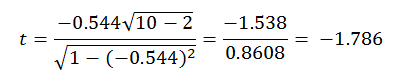
Because the absolute value of the resulting t-value is less than the critical value of t with 8 df , which with with 8 df an α of 0.05 is 2.306, you would now fail to reject the null hypothesis. There was insufficient evidence to conclude that the number of hours worked influenced quiz scores.
7.7 The reason that the correlations between quizmark and Zquizmark and between hoursworked and Zhoursworked equals 1.0 is that the transformation of a set of scores into the equivalent z-scores is a linear transformation. A linear transformation changes the absolute values of the scores but not the relative positions. Their rank ordering and the relative distances between them remain the same. Thus, the correspondence between the original scores and the z-scores is perfect.
The correlation in both cases is −0.544. Again, z-scores are merely linear transformations of the original scores. The absolute values of the z-scores change but not their relative positions, thus the correlation with either the original scores or the z-scores of the other variable will result in the same r.
7.10 The key to creating a data set where taking the third variable into account increases the strength of the correlation is to create two groups, both of which have a strong correlation between x and y. One group, however, should have a significantly great mean on the y-variable than the other. The example below illustrates the condition.
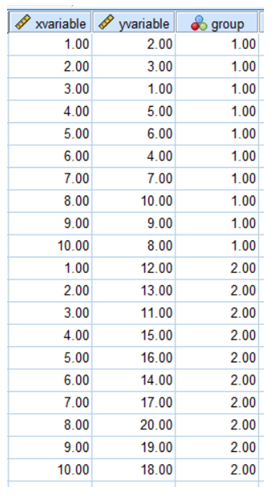
The overall correlation between the x-variable and the y-variable is 0.44. When the two groups are analysed separately the correlation in both cases is augmented to 0.88. Other outcomes are possible, particularly when multiple groups are amalgamated. A near-zero overall correlation can become a positive correlation when a pairing of two of the three groups is analysed, and the zero correlation can become a negative correlation when another pairing is amalgamated and analysed. Again, this is possible when the groups have different means on the y-variable.