Chapter 12: Multiple Regression
Short answer questions.
1. If we had one criterion variable and two predictor variables, what would be the differences between conducting a single multiple regression analysis and conducting two separate simple regression analyses and summing the results?
Main Points:
- If the predictors were completely independent, the R2 would simply be the sum of the two r2.
- If the predictors were completely independent, the slopes of the two predictors would not change.
- If the predictors were not completely independent, the R2 would be overestimating the sum of the two r2.
- If the predictors were not completely independent, the two slopes would likely change.
2. In terms of R2, when would there be no difference between running the two separate regressions and a single multiple regression as described in question 1? Why?
Main points:
- When the predictors are independent: all correlations among the predictors are 0.0.
- Because there is no overlapping of the variance in the criterion explained by the predictors, their effects can be added. Nothing will be summed more than once.
- It is similar to summing the sum-of-the-squares for the various treatment variables in a factorial ANOVA.
3. What is multicollinearity and what are the circumstances that produce it?
Main Points:
- Multicollinearity exists when a predictor is a linear function of other predictors.
- When a predictor is a perfect linear function of other predictors the analysis becomes impossible.
- There are various ways in which multicollinearity can be produced. (1) A predictor variable is highly correlated with one other predictor in the model. (2) A predictor variable is moderately correlated with a few other predictors. (3) A predictor variable is somewhat correlated with a number of other predictors. (4) Some combination of the above three is also possible.
4. What are four possible strategies for addressing multicollinearity?
Main Points:
- If there is only one predictor variable with a very low tolerance, then remove that variable from the model.
- If the source of the problem is a single high correlation with one other predictor, then one of the two variables may be excluded from the model.
- Alternatively, if the source of the problem is a high correlation with one other predictor, the two variables may be combined.
- Multicollinearity may also be addressed through a Step-Wise regression.
5. What are the three questions regarding possible interactions and how are they addressed?
Main Points:
- Is there an interaction? If there is an interaction, what is its strength? If there is an interaction, what is its nature?
- The presence is tested for by including the interaction term in the regression model and examining the possible significance of the interaction term in the coefficients table.
- The strength can be estimated by the difference in the R2 between the model that includes the interaction term and the model without the interaction term.
- Examining the nature of the interaction usually begins with a test for a bilinear interaction. A bilinear interaction exists when the B of one measurement predictor changes as a function of the scores on a second measurement predictor. Other types of interaction are also possible.
6. What is the difference between Missing at Random (MAR) and Missing Completely at Random (MCAR)?
Main Points:
- Data are MCAR when the missing values are unrelated to the other observed values of that variable and to all other observed variables in the study. For example, the missing values of a variable show no tendency to be related to high or low scores in another variable.
- A weaker assumption is that the data are missing at random (MAR). When data for a particular variable are MAR the missing data are deemed random with respect to the variables’ observed values, after controlling for the other variables used in the analysis. For example, scores on variable A could be assumed MAR if those subjects with missing variable A scores do NOT have on average higher or lower variable A scores than the subjects whose data are not missing. It is impossible to actually test the MAR assumption because we do not know the missing values thus we cannot test them against the observed values.
7. What are four possible strategies for addressing missing data?
Main Points:
- List-wise deletion of subjects with missing data is a common strategy. Many researchers fail to recognize that list-wise deletion often biases the results when the assumption of MCAR is violated.
- A second strategy is pair-wise deletion. This approach is based on the fact that linear regression analysis can be conducted without the raw data. All that is required are the means, standard deviations, and the correlation matrix.
- The third strategy, imputation, is actually a collection of techniques. In statistics, imputation means replacing the missing data with a reasonable estimate. Historically one of the first forms of imputation was to replace any missing value with the observed mean of that variable.
- Another form of imputation involves conducting a multiple regression(s) to replace the missing data prior to running your intended multiple regression.
Data set questions.
1. Create a data set in SPSS (n =10) with a criterion and two predictors where the presence of a multivariate outlier substantially affects the results. Demonstrate the effect by removing the outlier and rerunning the regression.
Main Points:
- The multivariate outlier needs to go against the trend of the relationship between the two variable.
- The Mahalanobis X2 value should be much larger than the critical value.
- This demonstration is easier to create when the sample size is relatively small. (The outlier will have a larger influence on the outcome.)
2. (A fictitious study) A researcher examined the existing literature on happiness and has proposed the following model of happiness. He deemed work to be important. The more we feel productive at work the happier we will be. He deemed pleasure to be important. Pleasure is defined as fun and the more fun we have the happier we will be. The literature also indicated to him that there may be an interaction between work and pleasure. Finally, he deemed openness to everyday experience important. Being able to enjoy the moment, any moment, simply for itself, appeared to him as crucial to real happiness. He called this the Zen factor, for lack of a better term. The psychologist tested a large number of subjects using psychometric tests of these variables. The data are listed in the file happinessstudy.sav on the texkbook’s web page. The predictor variables are age, work, pleasure, and zenatt. Happiness (Regr factor score) is considered the measure of overall personal happiness and is the criterion variable. What is the best model of happiness that you can derive from his data? Be sure to address the issues of missing data, tests for all types of outliers, linearity, multicollinearity, and a test for the normality of the residuals. Present a final model (with or without interaction term) along with the R2, the adj R2, and the individual regression coefficients (slopes). Also include any conclusions you wish to make. What limitations do you see with respect to your analysis and findings?
Mains Points:
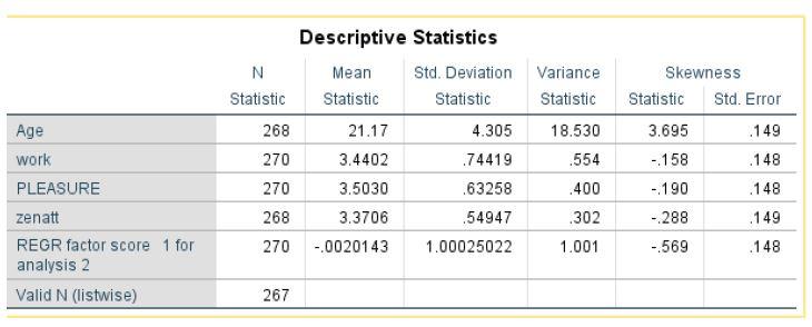
- Descriptive statistics are run. Z-scores are saved for each variable and no univariate outliers are found (no z-scores greater than 4.0 found in the new variables.)
- Scatter plots are run for the four predictors and the criterion. The relations appear linear and it appears that homoskedasticity can be assumed. For example, Happiness regressed on Zenatt.
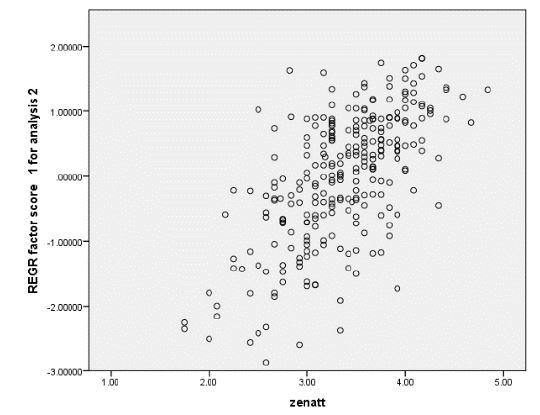
Age is the exception. Because it is nearly a constant, the scatterplot indicates that the variable has no linear relation with happiness and cannot be used in the regression.
- Happiness is regressed on work, pleasure, and zenatt. Mahalanobis values are saved to test for multivariate outliers. The ANOVA table indicates that the overall model is significant. The coefficient table reveals that all three predictors make a significant contribution to happiness when the others are held constant.
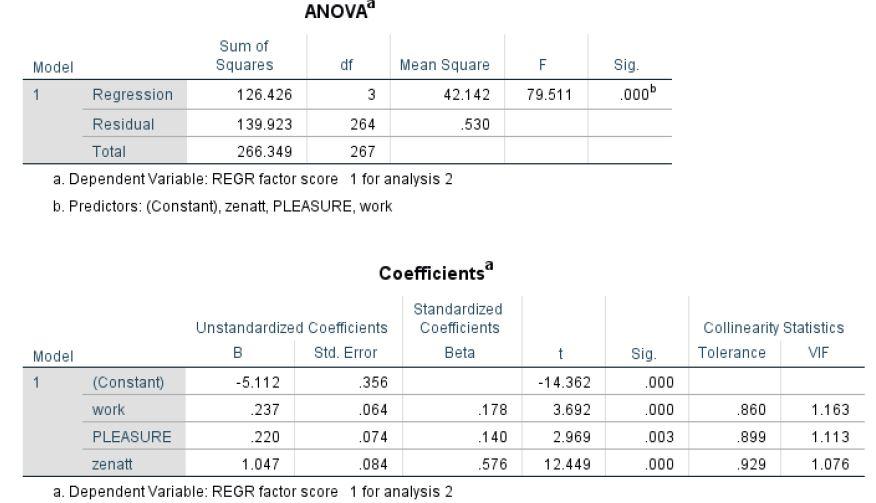
Tolerance values in the coefficients table indicate that there is no problem with multicollinearity.
d. Testing for an interaction between work and pleasure by creating a multiplicative term and including it in the model.
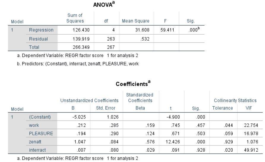
The interaction term is nonsignificant (t =.091, p = .928). Its presence had little effect on the other individual predictors. It merely reduced the overall explanatory power of the model.
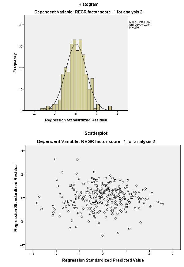
e. Regression for the standardized residuals on the standardized predicted values and the histogram indicate only minor issues with the normality of the residuals of the final model.
f. The best model, given the current data, is that work, pleasure, and zenatt all make an independent significant contribution to overall happiness.
