8.1 The independent variable is the cage condition in which the hamsters are housed for 30 days. The dependent variable is the number of middle squares that a hamster enters during the two-minute session.

8.3 There is no difference between the means of the three cage conditions is the null hypothesis with respect to difference. There is some difference between the means of the three conditions is the alternate or experimental hypothesis with respect to difference. ‘There is no association between the scores and the number of hamsters raised in a cage’ is the null hypothesis with respect to association or relation. ‘There is a relation or an association between the scores and the number of hamsters raised in a cage’ is the alternate or experimental hypothesis with respect to association.

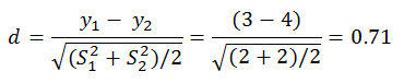
8.4 As discussed in earlier chapters, the effect size for a difference between two means is typically expressed as Cohen’s d, which is the difference between the two means divided by the pooled standard deviations. If the ns are equal, then

Using the effect size table in the Power appendix B table B1 we see that this is between a medium and a large effect.

Using the sample size table in the Power Appendix B table B2 we find that if we wished to test for a medium effect with a power of 0.8 we would need 64 hamsters per condition. If we wished to test for a large effect with a power of 0.8 we would need only 26 hamsters per condition.

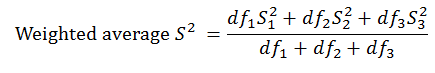
8.5 If the ns are unequal we would need to calculate the sum of squares for each condition and sum them and divide that total by the sum of the degrees of freedom across the conditions. Each variance can be multiplied by its degrees of freedom to reproduce the sum of squares. (The number of degrees of freedom for a condition is the number of observations minus one.) The sum of squares from all of the conditions can be summed. All of the degrees of freedom can be summed. The total sum of squares is then divided by the total degrees of freedom. This would provide the weighted average or best estimate of the population variance:

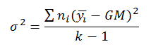
8.6 If the ns were unequal, n would not be a constant and you would need to move inside the summation sign. Each difference between a condition mean and the grand mean would need to be multiplied by the number of observations in each particular condition:

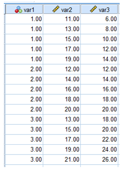
8.9 Begin by creating a three-condition data set with five observations in each condition. One of the observations in each condition will act as the mean. Then add the other four observations around the mean in a symmetrical fashion, for example, 1, 3, 5 (mean), 7, and 9. Compute the two independent estimates of the population variance, one based on the variance among the means and the other based on average within-condition variance. If the estimate based on the variance in the means is greater than the estimate based on the within-condition variance, then move the means closer together (linear transformation of the data, adding or subtracting a constant from the scores in a condition) and recompute the estimates. Repeat this linear transformation until the estimate based on the within-condition variance is greater than the estimate based on the variance among the means. If the estimate based on the variance in the means is less than the estimate based on the within-condition variance, then move the means further apart and recompute the estimates. Repeat this linear transformation until the estimate based on the within-condition variance is less than the estimate based on the variance among the means.

Below is an example. Variable 1 is the condition; variable 2 is a data set in which the estimate based on the variance in the means is the greater of the two estimates; variable 3 is a data set in which the estimate based on the within-condition variance is the greater of the two estimates.

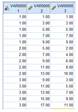
This illustrates the independence of condition variances and their means.

8.10 Begin by creating a three-condition data set with five observations in each condition. One of the observations in each condition will act as the mean. Then add the other four observations around the mean in a symmetrical fashion, for example, 11, 13, 15 (mean), 17, and 19. To produce the non-significant data set keep the means close together (e.g., 14, 15, and 16). Compute the F-value. Next create the significant data set while keeping the grand mean and the variances constant. Move the scores for the condition with the greatest mean further away from the middle condition by adding a constant to all of the scores. Move the scores from the condition with the lowest mean away from the middle condition by subtracting the constant that you added to the scores in the previous step. Run the ANOVA. If the resulting F-value is still non-significant, repeat the linear transformations until the F-value is significant.

Below is an example. Variable 1 is the condition; variable 2 is a data set in which the F-value is non-significant; variable 3 is a data set in which the F-value is significant. This exercise illustrates the independence of the condition means and the condition variances. Using var2 produces a non-significant F-value of 0.5. Using var3 produces a significant F-value of 18.0. How might you change the F-value in the second data set from significant to non-significant without changing the condition means?

8.11 An ANOVA summary table is made up of columns for the source, sum of squares, degrees of freedom, mean square, F, and p-value. If we assume that we know SS_treatment to be 40 and the F-value to be 5.0, we are unable to complete the ANOVA summary table. The crucial problem is that we have no idea of the degrees of freedom or the other sum of squares. Assuming that we know the SStreatment to be 40 and the F-value to be 5.0, if we know that there were 3 conditions and 15 subjects we would now have sufficient information for completing the table. There must be two df_treatment. This means that the MS_treatment must be 20 (40/2). In order for the F-value to be 4, the MS_error must be 5 (20/5). If there are 15 subjects, there are 14 df_total. If there are 14 dftotal and 2 dftreatment there must be 12 df_error. If there are 12 dferror and the MSerror is 4, the SS_error must be 60. If the SSerror is 60 and SStreatment is 40, the SS_total must be 100. This is all made possible by the fact that the sums of squares are additive and the mean squares are the sums of squares divided by the degrees of freedom. Finally, if you consult a F-table for α = 0.05, you will find that with 2 and 12 degrees of freedom the critical F-value is 3.89. Thus, the probability of an observed F-value (4.0) is less than 0.05.

8.13 The hamster data are best considered ratio in nature. Assume that the number of middle squares entered in the open-field test is at least interval in nature. That is, the difference between any two adjacent scores (e.g., 4 and 5) is equal to the difference between any other pair of adjacent scores (e.g., 7 and 8). Because there is a true zero – it is possible for a hamster to not enter any middle squares – the data can be considered ratio in nature.