Short answer questions.

1. What is the difference between a priori and post hoc follow-up tests?
Main Points:

1. A priori implies that the test was designed in light of previous research and knowledge of the topic.
2. A priori test are designed prior to data collection. There was the intent of conducting particular follow-up tests.
3. With post hoc tests the thought of making a particular comparison(s) did not arise until the researcher, at least cursorily, examined the collected data. We might call these “after the fact” comparisons.
4. The important point is that the intent of making the post hoc comparison(s) did not arise out of prior theoretical of empirical knowledge.

2. As a follow-up test, what advantage does the multiple t-test procedure have over simply carrying out a series of standard t-tests?
Main Points:

1. More efficient estimate of population variance because it is based on all condition variances found in the study, not only two.
2. Because as the degrees-of-freedom increase the statistical power increases.

3. In terms of their minimum-difference values, what is the difference between the Newman-Keuls, the Tukey’s HSD, and the Tukey’s WSD (B) tests? What statistical issues are behind the development of these tests?
Main Points:

1. All three tests compare all possible pairs of means.
2. The Newman-Keuls test reduces the critical value as the number of means between rank-ordered means decreases.
3. Tukey’s HSD used what would be the largest Newman-Keuls critical value for all pair-wise comparisons.
4. Tukey’s WSD uses as critical value the average between those that would be used by Newman-Keuls and those that would be used by the Tukey HSD.
5. A tension exists between avoiding a Type I error and avoiding a Type II error.
6. The Newman-Keuls offers the most power but the least Type I protection.
7. The Tukey HSD offers the most Type I error protection, but the least power, should the null hypothesis be false.
8. The Tukey WSD is a compromise.

4. What is the Holm-Bonferroni multi-stage procedure and how is it different from the standard multiple t-test procedure?
Main Points:

1. Where in the case of the standard multiple t-test procedure the per comparison alpha (critical value) is fixed, in the Holm-Bonferroni multi-stage test the alpha (critical value) can change.
2. The Holm-Bonferroni multistage procedure is a multiple t-test with a twist, allowing for a systematic reduction in the operative size of the family of comparisons, thus altering the pcα. First, calculate all of the planned t-tests using the multiple t-test formula.
3. Arrange the observed t-values from largest to smallest in magnitude.
4. Compare the p-value of the largest of the observed t-values to the appropriate critical p-value.
   
   1. The appropriate critical p-value is the desired fwα, typically .05, divided by the number of planned multiple t-tests in the family (family size).
5. If and ONLY if the observed t-value has a p-value less than the critical p-value for that particular family size do you advance to test the next largest t-value.
6. If the previous t-value had a p-value less than the critical p-value, then reduce the family size by one and return to step #4.
7. If you reach an observed t-value with a p-value greater than the critical p-value, then you conclude that this contrast and all contrasts with smaller t-values are non-significant.

5. Why are tests for polynomial trends not possible when the independent variable is qualitative in nature?
Main Points:

1. When the independent variable is qualitative, the numbers assigned to the various level are nominal only.
2. The numbers assigned to the levels of the independent variable can be swapped or changed in any way.
3. With one set of numbers assigned to the independent variable the trend may look linear.
4. With another set of numbers assigned to the independent variable the trend may look quadratic.
5. This is not the case when the independent variable is quantitative and the values represent an amount. 

Data set questions. 

1. Using 30 subjects (10 in each of three conditions), a psychologist tested the effects of caffeine on the Klutz Hand-Eye Coordination Test. In condition I subjects were given no caffeine. In condition II subjects were given 10 mg of caffeine. In condition III subjects were given 20 mg of caffeine. The psychologist wished to know if scores would simply improve linearly as the dosage was increased or if performance would suffer at higher dosages. The means for condition one, two, and three respectively were 20, 70, and 40 (the higher the score, the better the performance). The mean-square-error from the overall analysis was 125. There is no need to test assumptions or make a figure. You need only to carry out the statistical tests necessary to answer the psychologist’s questions and draw appropriate conclusions.
Main Points:

1.  
2. Weighting coefficients for a straight line and a quadratic trend are (-1,0,+1) and (-1, 2, -1), respectively.
3. Mean Square Linear is 2000.
4. Linear trend F-value is 16.0 (significant), reject the null hypothesis, sufficient evidence of a linear trend.
5. Mean Square Quadratic is 10,667.
6. Quadratic trend F-value is 85.3 (significant), reject the null hypothesis, sufficient evidence of a quadratic trend.
7. There is evidence that as the dosage was increased performance suffered at the higher dosage.

2. A driving safety officer tested the effect of sleeplessness on driving errors. She suspected that the longer drivers go without sleep after 24 hours, the more likely they are to make errors. She did not think that there would be an increase in errors until the 24 hours. She had twelve young adult drivers stay awake for 18 hours (Condition 1), 24 hours (Condition 2), and 30 hours (Condition 3). She then tested each of them on a driving simulator. The table below depicts the number of errors committed by each driver. Using a nonparametric test, do the data support her suspicion?

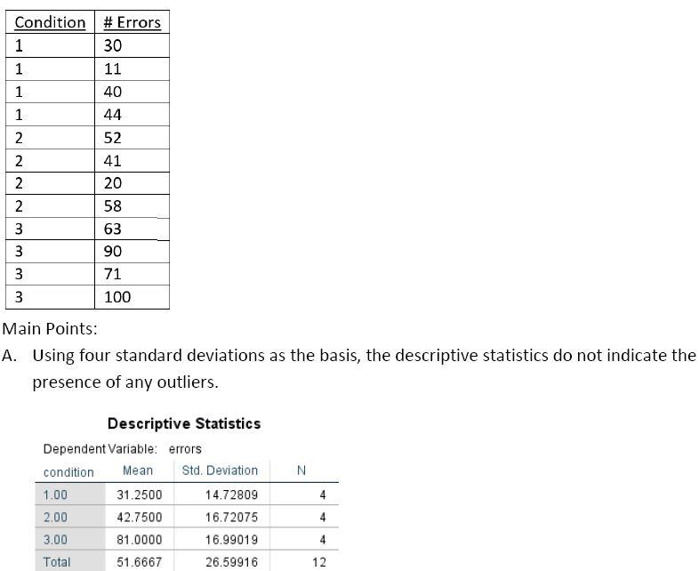
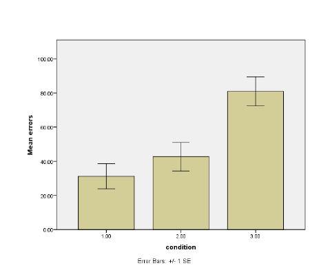
B. The graph indicates the general trend expected by the researcher. The group that went thirty hours without sleep appears to have made more errors that the other two groups.

 

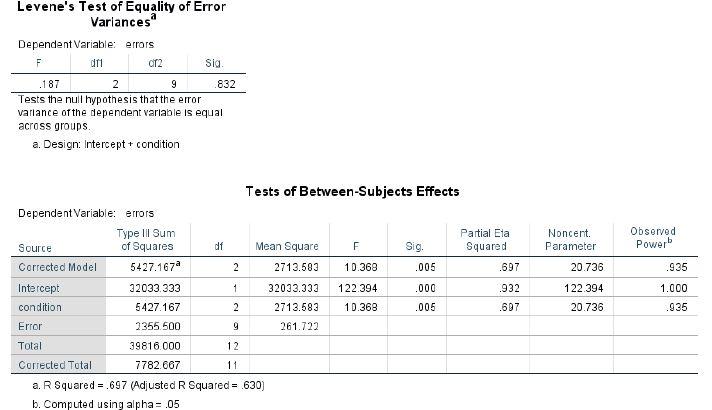
C. The Levene test is non-significant (p. = .832) indicating that homogeneity of variance can be assumed.
D. The null hypothesis regarding the effect of hours without sleep is rejected. Condition (hours without sleep) is found to be significant: F=10.368, MSE = 2713.583, p. = .005. The Partial Eta Squared reported by SPSS is .697. A computed Eta Squared would be (5427.167/ 39816.000) .14.

E. Difference contrasts indicate that condition 1 and 2 were not significantly different (contrast estimate = 11.5, p. = .341.), but, as predicted, condition 2 and 3 were significantly different (contrast estimate = 44.0, p. = .002).

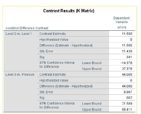
F. The result are as predicted by the researcher. The researcher had predicted that there would be an increase in driving error after going 24 hours without sleep.

3. A student completing a master’s degree in Animal Science is interested in the social behaviour of cats. From his experience he believes that cats that were previously outdoor cats and later became indoor cats would wish more attention from their owner than cats that had always been indoor cats. Furthermore, he thinks that cats that were always indoor cats but were the only cat in the household would wish more attention than cats who lived with litter mates. To test his ideas, the student asked five cat owners in each of the conditions to observe and report the number of times the cat sought attention over a 24-hour period. Do the data tabled below support the student’s suspicions? The scores represent the number of times during a 24-hour period the cat sought attention from its owner. Be sure to start with descriptive statistics, tests of assumptions, a graph, and an omnibus test. This is to be followed up with appropriate a priori tests.

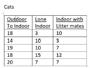
Main Points:
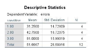
A. Using four standard deviations as the basis, the descriptive statistics do not indicate the presence of any outliers in any of the three groups of cats.

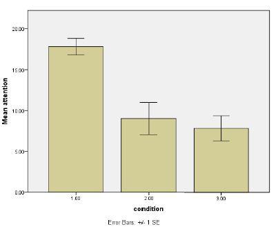
B. The figure appears to confirm that the cats that were outdoor cats at first required more attention from their owners than cats that had been indoor cats. However, there does not appear to be a difference between the “only” cats and the cats who lived with litter mates.

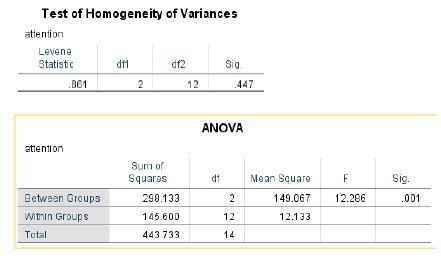
C. The Levene test is non-significant (p. = .447) indicating that homogeneity of variance can be assumed.
D. The null hypothesis regarding the effect of condition is rejected. Condition (hours without sleep) is found to be significant: F=12.286, MSE = 298.133, p. = .001. A computed Eta Squared would be (298.133/ 443.733) .67

E. As predicted by the researcher, the contrasts indicate that the cats in condition 1 were significantly different from the amalgamation of those cats in conditions 2 and 3: t = 9.4, p. = .001.). However, the “only” cats were not significantly different from those living with litter mates: t = .545, p. = .596).
F. The result partially support the researcher hypothesis concerning which cats would require more attention from their owners.