Short-answer questions.

1. From the model approach we have taken, given a repeated-measures design (one treatment variable), an individual observation in a given condition is composed of what components?
Main points:

1. Population mean
2. Treatment effect (if any)
3. Subject effect
4. Error

2. How are the components from question #1 estimated?
Main Points:

1. Population is estimated by the Grand Mean
2. A treatment effect is estimated by the difference between the mean of the treatment condition and the Grand Mean.
3. A subject Effect is estimated by the difference between the mean of the subject’s scores and the Grand Mean.
4. Error is estimated by subtracting the treatment condition mean and the subject mean from the subject’s score and adding the Grand Mean. 

3. What comprises the sum-of-squares between-subject in a repeated-measures analysis?
Main Point:

1. All individual differences at the time of testing.

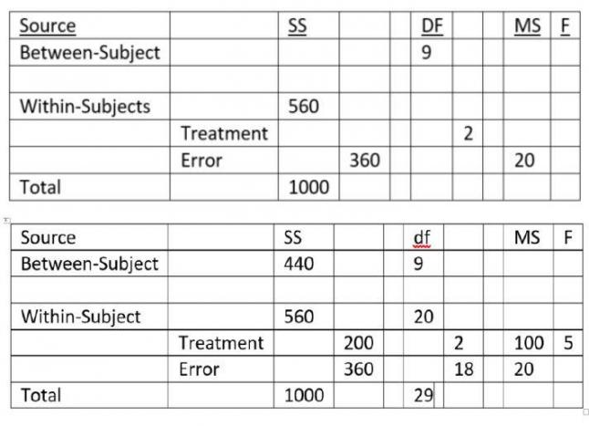
4. Complete the below repeated-measure ANOVA summary table. 

5. What could happen to the sums-of-squares, the mean-squares, the degrees-of-freedom (total, treatment, and error), and the F-ratio if a data set that was first analysed as a between-subject design was subsequently re-analysed as a repeated-measures design? (Be sure to cover all categorically different outcomes.)
Main Points:

1. Assume that there are substantial individual differences.
   1. The sums-of-squares, the mean-squares, the degrees-of-freedom total and treatment would be unchanged.
   2. The sums-of-squares, the mean-squares, the degrees-of-freedom error would change. The degrees-of-freedom error would be reduced by the number of subjects minus one.The sum-of-squares error would be reduced by the sum-of-squares between-subjects.To the extent that the sum-of-squares errors was reduced in greater proportion than the degrees-of-freedom error, mean-square error would be reduced and the F-ratio would increase. (increase power)

 B. Assume that there are virtually no individual differences.

1.  The sums-of-squares, the mean-squares, the degrees-of-freedom total and treatment would be unchanged.
2. The sums-of-squares error would remain virtually unchanged.
3. The degrees-of-freedom error would be reduced by the number of subjects minus one. To the extent that the degrees-of-freedom error was reduced in greater proportion than the sum-of-squares error, the mean-square error would increase and the F-ratio would decrease. (loss of power)

6. How do we ensure that block and treatment are kept independent in a randomized-block design? Why is that necessary?
Main Points:

1. An equal number of members of all blocks are assigned to all treatment conditions.
2. This prevents any confounding of treatment and block effects.

7. When is it most appropriate to use Friedman nonparametric test for related-samples?
Main Points:

1. When a researcher’s data are not measurement in nature.
2. In other instances where the assumptions cannot be met or violations not easily evaluated or corrected. 

Data set Questions

1. First, imagine an analysis of a data set with three conditions and 5 observations in each condition. The Sum-of-squares total, treatment, and error are 73.6, 19.6, and 54, respectively. The degrees-of-freedom are 14, 2, and 12 respectively. Assuming a between-subject design, what is the resulting F-value and what do you conclude? Now imagine a blocking variable that accounts for 50% of the sum-of-squares total. What is the new resulting F-value and what do you conclude?
Main points:

1. Mean-Square Treatment = (19.6/ 2) = 9.8
2. Mean-Square Error = (54/12) = 4.5.
3. F value = (9.8/4.5) = 2.18. Critical F-value = 3.89.
4. We fail to reject the null hypothesis and conclude that there is insufficient evidence that the independent variable influences the dependent variable.
5. New Sum-of-Squares Total is 73.6(.5) = 36.8.
6. New Sum-of-Squares Error is 36.8 – 19.6 (sum-of-squares treatment) = 17.2.
7. New degrees-of-freedom error is 11
8. New Mean-Square Error is 17.2/11 = 1.56.
9. The new F value is (9.8/1.56) = 6.28.
10. Reject the null hypothesis (critical F-value = 3.98). There is sufficient evidence to conclude that the independent variable influences the dependent variable.

2. Construct a data set of 15 whole numbers between 5 and 20. Separate them into three equal groups (treatment conditions) twice. In the first data set, the resulting between-subject F-value should be nonsignificant but the repeated-measures analysis of the data should be significant. . In the second data set, the resulting between-subject F-value should be significant but the repeated-measures analysis of the data should be nonsignificant.
Main Points:

1. The first part of this question is fairly simple. Insure that there are substantial individual differences (differences in subject means).
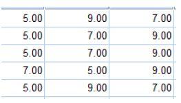
2. The second part requires that you reverse the trend. There should be almost no differences in the subject means. When this is the case you will lose degrees-of-freedom error by no sum-of-squares error. This will result in a loss of power. If you design the between-subject analysis such that the results are barely significant, the within-subject analysis should have a p-value greater than .05.
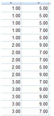
3. Here is an example of the data for the second part organized for a within-subject analysis and a between-subject analysis. 

 

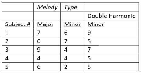
3. The below table represents 5 subjects who rated (on a 1 to 10 scale) a melody played three different ways: once in a major key, once in a minor key, and once in a double harmonic minor key. Because the subjects were of Hungarian origins the researcher thought that the double harmonic minor version of the melody would be rated the highest. Do the data support his hypothesis?

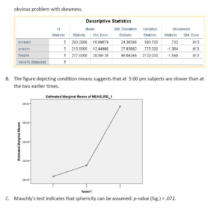
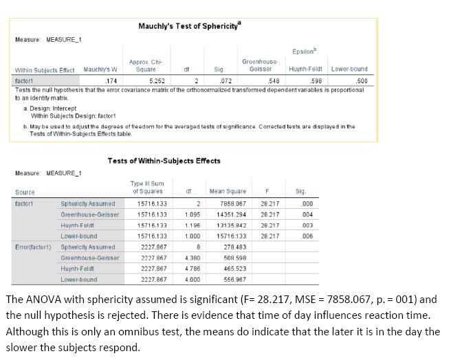
4. A psychologist noticed that, relative, to the number of cars on the road, there were more accidents in the afternoon than in the morning or mid-day. He suspected that time of day affected reaction time (RT) , and slightly slower RTs were responsible for more accidents. He suspected that people were “psychologically” tired by the afternoon. To test his hypothesis, he tested the simple RTs of 5 subjects at 9:00 am, 1:00 pm, and 5:00 pm. The data are presented in the table below. Do the below data support the idea that RT is sensitive to time of day? RT is recorded in milliseconds. The greater the RT the slower the subject. Be sure to include all tests of assumptions (with conclusions), descriptive statistics, appropriate figures, test of overall null hypothesis, and ANOVA summary table.