12.3 The minimum score of ingenium is 17.0 and the maximum score observed was 45. If you wish to predict a mendax score for someone with an ingenium score between those two values, even if no one in your study had that particular score (e.g., 25), you could feel confident using the y-intercept (constant) of 25.207 and B of −0.298 for making the prediction. This is called interpolation. If, however, you wish to predict a mendax score for someone with an ingenium score below 17 or above 45, you can be less confident using your y-intercept and B. This is called extrapolation. Scores outside of the range of ingenium in your data need to be interpreted with care. The further below 17 or above 45 the ingenium scores are, the more likely there is a change in the nature of the relation with mendax scores.

12.5

Everything is derived from the correlation matrix,

so it better be stable!

You should try to work your way through this now. If you find it difficult, do not be surprised. The diagrams at the end stand almost on their own. After completing this chapter, the earlier parts of this link should be easier to follow.

I. Two predictors:

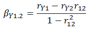
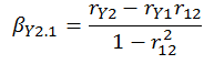
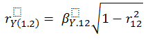
1. The standardized slopes or regression coefficients can be computed simply by knowing the relevant correlation coefficients (look at the denominator; it is the proportion of the variance that is not shared with predictor 2):

1. Your multiple R can be computed several ways. You may derive it from the simple correlations and their squares:

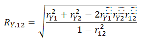
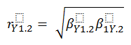
You may derive it from the standardized slopes:

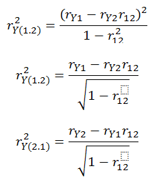
1. Semi-partial or part correlations are the square root of overall R² minus R² reduced by the variance in y accounted for by a second predictor. These are called semi-partial or part correlations because the variance of the second (controlled for) variable is removed from the predictor, but not from the criterion. Therefore, in the case of two predictors, the semi-partial correlations are equal to

Using the above equation and a bit of algebra you will discover the following. It is not easy to follow at first. Try to look at the pairs and see that they are only correlations. For example, in the numerator in the first equation below you begin by multiplying the correlation between the criterion and the second predictor by the correlation between the two predictors. You then subtract that product from the correlation between the criterion and your primary predictor. Finally, you square that difference.

Thus, from the relationship between the correlations and the standardized sloped we can derive the following:

1. Partial correlations differ from semi-partial correlations in that the overlapping (or covariance) variance is removed from both the criterion and the predictor.
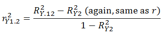
2. The partial correlation is equal to overall R² minus R² where the criterion is regressed on only the second predictor. This difference is then divided by 1 minus the R² that resulted from the criterion being regression on only the second predictor. In the two-variable case the equation is thus

Again using the above equation and some more algebra you will find the following:

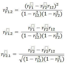
The relation between partial correlations and the standardized slopes can be viewed as follows:

Some authors say that the semi-partial or part correlations are directional and the partial correlations are non-directional. Thus, part correlations would be more appropriate when your theory involves a causal or directional prediction.

1. You might visualize these two types of correlations in terms of the following diagram of overlapping circles.

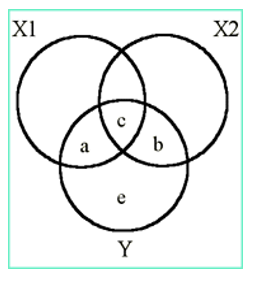
The total Y variance is a + b + c + e. In standardized terms this equals 1.0 or 100% of the variance in y.

The semi-partial or part correlations are that portion of a predictor variable (X1) that is shared with the criterion (area a) which, however, is not shared with the other predictor (X2) divided by 100% of y: that is, a/(a+b+c+e):

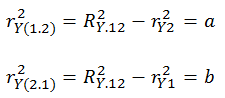
Partial correlations are that portion of a predictor variable (e.g., X1) that is shared with the criterion (area a) which is not shared with the other predictor (e.g., X2) divided by ‘area a’ plus that part of the criterion variable (y) that is not shared with X2 (area e) or a/(a+e):

Hopefully you will see how everything can be derived from the correlation matrix. Again, this illustrates the importance of its stability, which rests on the test–retest reliability of the individual measures with respect to the population that the sample is drawn from and, of course, the number of observations.

12.8 The p-values for the F-value in the ANOVA table and for the t-value in the coefficient table are identical. First, keep in mind that the t-value is the square root of the F-value. Thus, the test statistics are actually identical. Second, when there is only one predictor variable, the effect of the predictor is the same as the effect of the overall or complete model. In this case, the one predictor is the complete model. The ANOVA table reports the overall effect and the coefficient table reports the effect of the single predictor. When there are multiple predictors the p-values of any of the individual predictors are not likely to equal that of the F-value for the overall model.

12.12 The assumption of linearity is important for OLS regression. If the relation is curved it can lead to misleading predictions. When the relation is curved (e.g., inverted U-shape), using the OLS line to make predictions at all levels of x-axis values will result in overestimates or underestimate for the corresponding y-values. This depends where on the x-axis the x-value occurs. (See the discussion in an example in Chapter 7.)

In regression analysis we assume that the variance in the y-values is a constant along the regression line (homoscedastic) and is unrelated to the x-values. As an example, segment a regression line into three parts: the low x-values, the medium x-values, and the high x-values. A violation of the assumption of homoscedasticity (heteroscedasticity) would be indicated by the variability about the regression line differing across the three segments. For instance, there could be little variance in the y-scores at the low values on the x-axis, more variance at the medium x-axis values, and great variance at the high x-axis values. Or there could be little variance in the y-scores at both the low and high values on the x-axis, but considerably more variance at the medium x-axis values. Heteroscedasticity produces two common forms of distortion. First, the correlation coefficient will underestimate the strength of the association for some segments of the x-axis and will overestimate the association at other segments. Remember, visually r is a function of how near the points in the scatterplot are to the regression line. Second, the amount of error (standard error of the estimate) related to predictions will be underestimated for some segments of the x-axis, and it will be overestimated at other segments.

12.13 The more symmetrically the twenty values are distributed about their mean, the smaller the change in the recalculated means. The bigger change is in the variance. There is little change in the variance when one missing value is replaced by the mean. There is a considerable reduction in the variance when five missing values are replaced with the mean. Finally, there is a great reduction in the variance when the ten missing values are replaced with the mean. In conclusion, if a very small proportion of the data is missing, the strategy of replacing missing values with the mean will have little effect on any analysis. When a substantial proportion of the data is missing, however, replacing the missing values with the mean of the variable may significantly influence the results.

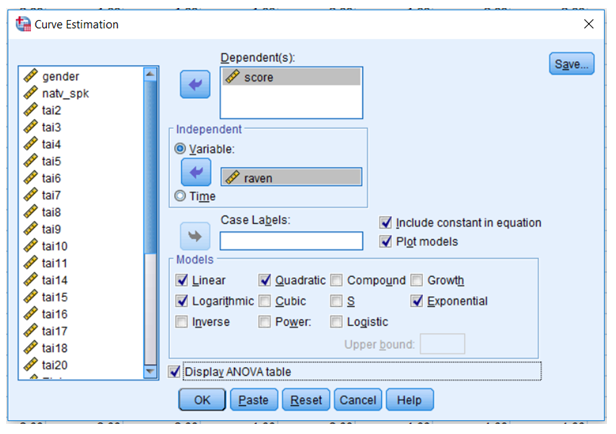
12.15 There are additional techniques for examining the linearity or possible nonlinearity of your data. In the Data Editor window for the multipleregressiondataset.sav data set, scroll down under Analysis to Regression and then move over and select Curve Estimation. Move score over to the Dependent(s) area and raven over to the Independent area. In the Models area select Linear, Quadratic, Logarithmic, and Exponential. This will allow you to evaluate these four possible relation between score and raven.

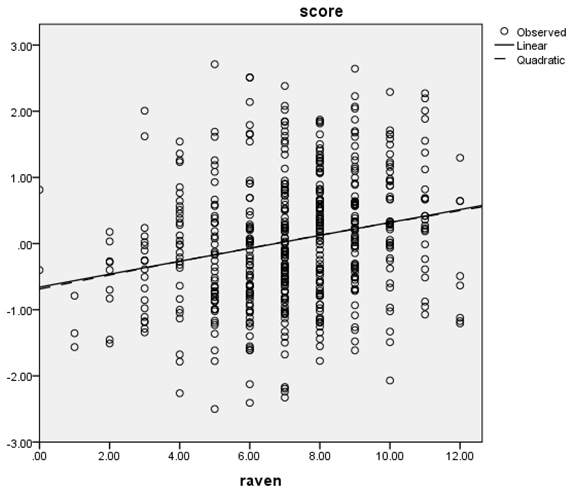
The first output we will examine is the Model Summary table. The only two trends that we were able to evaluate were the linear and the quadratic. Both were found to significantly ‘fit’ the data in the scatterplot. Does this mean that because of the significant quadratic trend we cannot assume linearity? Not necessarily. It is always important to examine scatterplots. 

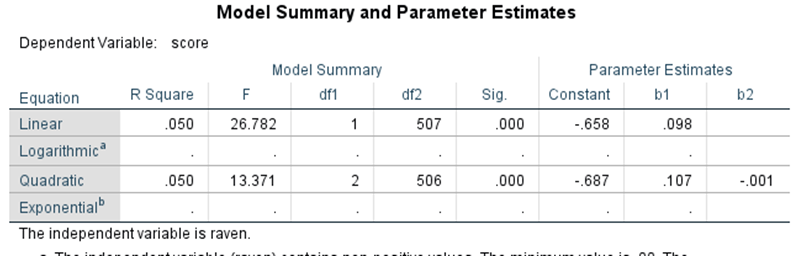
If we examine the scatterplot and the lines that depict the linear and quadratic trends, we see that there is minimal difference between the two trends. Although the quadratic trend was found to be significant, the scatterplot illustrates that the trend is very slight and is present only at the very extremes of the x-axis. In such cases, there is no need to treat the relation between the two variables as anything but linear. The very small quadratic trend can be found to be significant because of the number of observations: n = 539. Remember, p-value does not indicate effect size.

12.16 When score is regressed separately on Etai, R² = 0.15 and , and the overall model is significant: F = 8.064, p = 0.005. The regression coefficient and the standardized regression coefficient are −0.022 and −0.123, respectively. The t-value is −2.840, p = 0.005. When score is regressed separately on Wtai, R² = 0.082 and  and the overall model is significant: F = 46.630, p < 0.001. The regression coefficient and the standardized regression coefficient are −0.060 and −0.286, respectively. The t-value was −6.829, p < 0.001. When score is regressed simultaneously on Etai and Wtai,R² = 0.096 – nearly the same as the sum of the separate R²s (0.097) – and  The substantial change is in the regression coefficients. The regression coefficient for Etai is transformed from −0.022 to +0.30. The regression coefficient for Wtai is changed from −0.060 to −0.086. Both regression coefficients remain statistically significant. The perplexing finding is that the regression coefficient goes from being significantly negative to being significantly positive. To understand this we turn to the collinearity statistic of tolerance (0.484), which indicates possible distortions in the findings due to multicollinearity.

12.17 The variance inflation factor (VIF) is the reciprocal of tolerance. Thus, the tolerance for the three variables listed (Jockwins, Hands, and Horsewins) are (1/VIF) 0.189, 0.952, and 0.186, respectively. 

12.18 The are two basic forms of stepwise regression. The first, and most common form, is the forward selection approach, which we used in this chapter. This approach involves starting with no variables in the model. Then each predictor variable is tested using a chosen model fit criterion, which is the α level chosen by the researcher. Typically, the 0.05 or 0.01 level is chosen. Variables (if any) are added whose inclusion results in a statistically significant improvement and provides the largest increase in R². This process is repeated until no variables are found to statistically improve the model.

The other common form of stepwise regression is the backward elimination approach. This approach begins by including all predictor variables in the model. testing the deletion of each variable. Using a chosen model fit criterion, variables are deleted from the model based on whose exclusion results in a statistically non-significant deterioration yet provides the greatest decrease in R2. This is repeated until no further variables can be deleted without a statistically significant loss of fit for the overall model.

12.19 Because a hand is 4 inches, the regression coefficient in hands would be 4 (−0.21) or −0.84.

12.21 We will restrict this example to the approach that begins by creating a multiplicative term. Using the Create Variable option under the Transform tab in the Data Editor, create a new variable by multiplying natv_spk by Wtai of the corresponding factor score. Then regress score on natv_spk and Wtai. Regardless of which way you create the new multiplicative term, you will find that the regression coefficient for the interaction term approaches 0.0 and there is no increase in . Thus, you may conclude that there is no evidence of a bilinear interaction.