2.1 With which of the four scales of measurement did you associate the following measures?

1. Your year of birth. (Interval: The differences between adjacent years are equal, but our system of keeping track of the number of years does not have a true zero.)
2. Your marks in secondary school. (If the marks simply indicate the number of items answered correctly, then the marks are ratio in scale. They have a true zero as well as equal intervals between adjacent marks.)
3. Your shoe size and width. (Ordinal: It is not clear that adjacent shoe sizes all have the same difference in either length or width. But it is possible that the intervals are equal. There does not appear to be a true zero with respect to shoe size, thus the scale cannot be ratio.)
4. The number of the row in which you sat during the last lecture (from front to back). (Ordinal: Assuming that the rows are numbered from front to back, they do indicate the relative distance from the front of the room. Also, if the rows are equally spaced, then the numbers would be on a ratio scale with a true zero.)
5. Your income last month. (Ratio: Dollars, pounds, euros are all equal interval in scales. Furthermore, it is possible that you had no income last month.)

2.2 What is the difference between an experiment and a quasi-experiment?

In an experiment the independent variable is theoretically independent of all other variables. This is made possible by the fact that subjects can be randomly assigned to different conditions (groups). For example, subjects can be randomly assigned to the high-frequency word condition or to the low-frequency word condition as they walk into the lab. In a quasi-experiment the independent variable is not theoretically independent of all other variables. Subjects cannot be randomly assigned to different conditions (groups). The groups comprising the different levels of the independent variable are naturally occurring. For example, we cannot randomly assign subjects to a gender, an eye colour, or to a country of origin as they walk into the lab. Nor can we assign them to an income category or to a choice of occupation. Thus, in a quasi-experiment the so-called independent variable carries with it an innumerable number of confounding variables.

2.3 Below is some practice with the rule of summation notation that will facilitate following the basic definitional formulae that are used in the textbook. Keep in mind that summation notation is merely a way to indicate a repetitive process.

Summation notation: This is simply a system of shorthand for operations that are repeated with no change in variable(s), but a change in values.

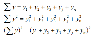
Rules of summation:

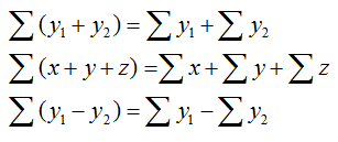
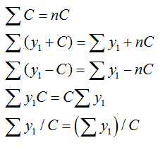
Where C is a constant:

2.4 For some practice with binning data for the creation of frequency histograms, open the binninghistogram1.sav SPSS file. When the file opens, select Graphs and slide down and click Chart Builder. Click OK when the new window opens. When the Chart Builder window opens, select Histogram from the Choose from area. Drag the leftmost example into the upper right area. Highlight and move the examscore variable to the x-axis. In the Element Properties Window click the Set Parameters button. When the Element Properties: Set Parameters window opens, choose the Custom bin size. Set the number of intervals to a desired setting. Click Continue. Click Apply on the Element Properties window and then OK on the Chart Builder window.

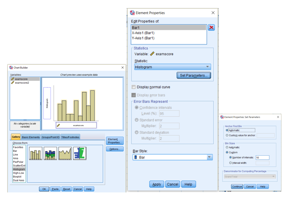
Try several settings for both examscore and examscore2.

Below are two examples:

1. Variable examscore with 10 and 5 bins.

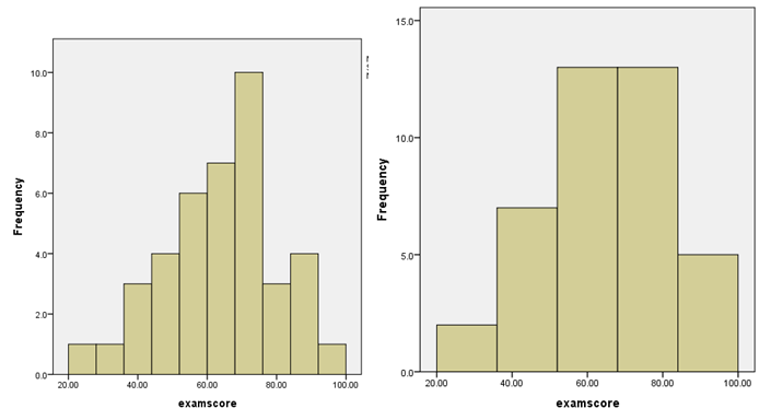
1. Variable examscore1 with 10 and 4 bins.

 2.5 

1. What is the minimum number of values you would need to change the median?

One! The score that is the median or closest to it. For example, if the scores were 1, 3, 5, the median would be 3.0. If we change the 3 to a 4, then the median would be 4.0. Changing either the 1 or the 5 would not change the median (e.g., 2, 3, 100).

2. How many values can you change without changing the median?

All of them! For example, add 1 to all of the values above the median and subtract 1 from all of the values below the median. The score in the middle will remain the score in the middle.

3. How many values can you change without changing the mean?

All except the mean, if the scores are symmetrically distributed about the mean. For example, add 1 to all of the values above the mean and subtract 1 from all of the values below the mean: change 3, 5, 7 to 1, 5, 9. In both cases the mean is 5.0.

4. Can you change the value of only one score without changing the mean?

No.

2.6 When will it make no difference whether we use the mean or the median for calculating the total absolute difference and the total squared difference?

When the distribution is normal, the median and the mean are the same value. Thus, it will make no difference which one is used for either calculation.

2.7  There are two types of circumstances where the sample ns are unequal and it is possible to calculate the grand mean by summing the means of the subgroups and dividing by the number of groups. Remember, the mean is the point that cuts the total value in half: half will be negative with respect to the mean and half will be positive. Also keep in mind the nature of a symmetrical distribution.

In the first case the sample means are all equal.

Sample 1: scores are 3, 4, 5; mean is 4

Sample 2: scores are 2, 3, 5, 6; mean is 4

Sample 3: scores are 3, 4, 5; mean is 4

The grand mean is 4.

In the second case the scores in two of the conditions are symmetrically distributed about the mean of the condition with the mean in the middle.

Sample 1: scores are 3, 4, 5; mean is 4

Sample 2: scores are 4, 5, 5, 6; mean is 5

Sample 3: scores are 5, 6, 7; mean is 6

The grand mean is 5.

2.8 In var2 there are no scores above the IQR. The whisker is equal to the top of the box. Why?

The scores are negatively skewed such that there are no scores above the 75% percentile.

Why are there no whiskers on the box for var3?

The scores are closely clustered and all fall within the IQR.

2.9 Why are the variances of the following two sets of scores the same?

Set A: 1, 2, 3.

Set B: 101, 102, 103.

The scores in the two sets are the same distance from their mean. Stated more formally, the sums of the squared distances from the mean are equal, as are the number of observations. The second set of scores is the first set with a constant added to all of the scores. When a constant is added to all of the scores in a set the mean is changed by the value of the constant, but the variance and standard deviation are unchanged.

Can you create a data set of five observation that has a mean of 3 and a variance of 4?

• A mean for five observations implies that the total of the scores was 15.
• A variance of 4 would require a sum of squares of 15 with 4 degrees of freedom.
• One such set of scores would be 1, 1, 3, 5, 5.

2.10 How is it possible that var1 and var3 can look so different in terms of their spread and have the same variance? 

Although the clustering of the scores is quite different, the average squared distance that the scores are from their means is identical. Clustering is independent of the average squared distance that the scores are from their mean. Related to this is the fact that so many procedures rely on the assumption that the distribution of scores is symmetrical (normal) about their mean. Also, variances are sensitive to outliers. On outlier in a very clustered set of scores can result in a variance that is similar to the variance of a set where the scores are more spread out, but without the outlier.

2.11 Both could be considered measures of spread. Begin with a set of scores: 2, 3, 4, 3, 4, 1, 4.

The average absolute difference (in the original units of measurement) between the scores and their mean (3.0) is 1.2. On the other hand, if we square the differences and then take the square root of the averaged sum, we arrive at a different answer (1.58). The important difference between the two measures of spread is that the standard deviation based on the squared differences is an unbiased estimator, but the average absolute difference is not. This difference is crucial for many statistical tests discussed in this book.

2.12 What would be the new mean and variance had we winsorized the score of 100 to three standard deviations above the mean rather than to four?

The new mean would be 7.945 and the new variance would be 177.25.

If you had a sample of four scores and the first three scores were 1, 2, and 3, how big would the fourth score need to be for it to be identified as an outlier? What does this problem teach us? Good luck! You will not find a number large enough to be considered an outlier. Remember, all four scores need to be used to calculate the mean and standard deviation. This points out the problem of attempting to identify outliers when the sample size is small. This and related problems, as well as possible solutions, will be addressed in detail in Part II of the book.

2.13 http://shocf.atwebpages.com/bors/textbook/index.html 

2.14 Challenge Question:

Would changing the numbers that label the categories in the above education-level example to 1, 3, 5, 7, and 9 change the median and IQV? If you think the change will alter the median and IQV, why and how? If you think the change will make no difference, why not?

No, it will not. The numbers on the categories are only names. The proportion of observations in the categories is the important issue, not the number used to name the category.

2.15 Challenge Question:

How does sample size affect the extent of bias when n rather than (n − 1) is used in the denominator of the variance formula?

The smaller the sample size, the greater the average bias in the estimate using only n in the denominator. As n increases, the amount of correction offered by using (n − 1) is reduced. When n equals 2, (n − 1) provide a 50% correction. When n equals 100, (n − 1) provides only a 1% correction.