Chapter 11: Comparisions of Means and Proportions

1. A statistics instructor is concerned that after her students perform well on the first of two major examinations in the introductory-level class, their performance appears to drop off on the second. Since this pattern appears to repeat itself across many sections of the same statistics class at her university, she wants to confirm that the downward trend in performance on the two 100-point examinations is real. To this end, she collects the examination results for a random sample of n = 12 students from the previous academic year. The scores on Exam 1 are: 79, 92, 81, 80, 79, 80, 78, 88, 86, 88, 77, and 93. On Exam 2, they are: 80, 75, 67, 82, 76, 71, 78, 78, 80, 77, 78, and 75. Create a data frame that organizes this data into two variables and 12 observations and use R to answer questions (b) and (c).

(a) Are these data independent or paired? Why?

Answer: Since there are two measurements on each of the 12 students, these data are paired.

(b) What is the point estimate of the difference between the two population means, µ₁ − µ₂?

Answer: 7

ex1 < c(79, 92, 81, 80, 79, 80, 78, 88, 86, 88, 77, 93)
ex2 <- c(80, 75, 67, 82, 76, 71, 78, 78, 80, 77, 78, 75)
scores <- data.frame(Exam1 = ex1, Exam2 = ex2)
scores
##     Exam1   Exam2
## 1      79         80
## 2      92         75
## 3      81         67
## 4      80         82
## 5      79         76
## 6    80 71
## 7    78         78
## 8    88         78
## 9      86         80
## 10    88         77
## 11    77         78
## 12    93         75
mean(scores$Exam1)
##   [1]   83.41667
mean(scores$Exam2)
##   [1]   76.41667

mean(scores$Exam1) - mean(scores$Exam2)
## [1] 7

Answer: The 95% confidence interval estimate of the difference in means is [2.41, 11.59]

t.test(scores$Exam1, scores$Exam2, conf.level = 0.95,
paired = TRUE)
##
## Paired t-test
##
## data: scores$Exam1 and scores$Exam2
## t = 3.3568, df = 11, p-value = 0.0064
## alternative hypothesis: true difference in means is not equal to 0
## 95 percent confidence interval:
## 2.410281 11.589719
## sample estimates:
## mean of the differences
## 7

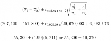
2. A recent study of the cost of living in various US cities has found regional differences in home prices. Two of the cities considered are Dallas, Texas and Minneapolis, Minnesota. The following data have been collected in the studies for those two cities: 47 homes in Dallas are for sale for an average of $151, 800, with a standard deviation of $17, 457; 34 comparable homes are for sale in Minneapolis for an average
of $207, 100, with a standard deviation of $26, 510.

(a) Are these data paired or independent? Why?

Answer: Since the Dallas data are collected independently of the Minneapolis data, they are independent.

(b) Find the 95% confidence interval estimate of the difference between the mean price for a home in Minneapolis and a comparable home in Dallas.

Answer: $55, 300 ± $10; 370 or [$44, 930; $65, 670]

qt(0.025, 79, lower.tail = FALSE)
## [1] 1.99045

3. The data set temps can be found on the book website. The two variable names are Daytemp and Nighttemp, and report the high (Daytemp) and low (Nighttemp) temperature in degrees Celsius for 10 European cities. The data are displayed below. Use R to answer parts (b) and (c).

temps
##                City                     Daytemp                    Nighttemp
## 1         Athens                 21                               12
## 2          Barcelona                   12                                9
## 3                Dublin                     6                                1
## 4         Lisbon                   15                                 9
## 5     Luxembourg                   3                                -2
## 6        Moscow                   2                                 1
## 7            Munich                    4        -2
## 8              Naples                  14                                11
## 9           Paris                    7                                -1
## 10      Stockholm                    2                              -4

(a) Are these data independent or paired? Why?

Answer: Since there are two measurements on each city, these data are paired.

(b) What is the 90% confidence interval estimate of µ₁ – µ₂?

Answer: The 90% confidence interval estimate of µ₁ – µ₂ is [3.812, 6.588].

t.test(temps$Daytemp, temps$Nighttemp, conf.level = 0.90,
paired = TRUE)
##
## Paired t-test
##
## data: temps$Daytemp and temps$Nighttemp
## t = 6.8675, df = 9, p-value = 7.328e-05
## alternative hypothesis: true difference in means is not equal to 0
## 90 percent confidence interval:
## 3.811989 6.588011
## sample estimates:
## mean of the differences
## 5.2

Answer: Since p-value = 0.00007 < α = 0.10, we reject H₀ : µ₁ – µ₂ = 0.

t.test(temps$Daytemp, temps$Nighttemp, conf.level = 0.99, paired = TRUE)

## Paired t-test

## data: temps$Daytemp and temps$Nighttemp

## t = 6.8675, df = 9, p-value = 7.328e-05

## alternative hypothesis: true difference in means is not equal to 0

## 99 percent confidence interval:

## 2.739264 7.660736

## sample estimates:

## mean of the differences

## 5.2

4. During two recent tax years, the US Internal Revenue Service (IRS) conducted an in-house investigation of the accuracy of tax lling advice given by IRS agents to individuals who call with questions about how to handle various tax issues. During the first phase, conducted in 2013, 900 calls were placed to IRS offices for tax advice, and after reviewing the accuracy of the advice provided, the investigation found that on 82 occasions the advice was incorrect. In a follow-up investigation in 2014, 800 calls were placed and on 28 occasions the advice was incorrect. Does it appear that the IRS has successfully improved the accuracy of the advice provided by its agents from one year to the next? Use R to find the 95% confidence interval estimate of p₁– p₂ and use R to check the result.

Answer: 0.0561 ± 0.0227 or [0.0334, 0.0788]

bad <- c(82, 28)

total <- c(900, 800)

prop.test(bad, total, conf.level = 0.95, correct = FALSE)

## 2-sample test for equality of proportions without continuity

## correction

## data: bad out of total

## X-squared = 22.034, df = 1, p-value = 2.679e-06

## alternative hypothesis: two.sided

## 95 percent confidence interval:

## 0.03340345 0.07881877

## sample estimates:

## prop 1 prop 2

## 0.09111111 0.03500000

5. In a recent consumer confidence survey of 400 adults, 54 of 200 men and 36 of 200 women expressed agreement with the statement, "I would have trouble paying an unexpected bill of $1, 000 without borrowing from someone or selling something." Do men and women differ on their answer to this question? Use the six-step framework to test H₀ : p₁ – p₂ = 0 against H_a : p₁ – p₂ ≠ 0 at the α = 0.05 level of significance. What is the p-value? Use R to confirm your answers.

(a) Develop the null hypothesis in statistical terms.

Answer: H₀ : p₁– p₂= 0

(b) Develop the alternative hypothesis in statistical terms.

Answer: H_a : p₁– p₂ ≠ 0

Answer: α = 0.05

n₁ = 200 and n₂ = 200

(d) Use α to specify the rejection region RR.

Answer:

where

and where

and
p-value = p(z>2.1553) + p(z<– 2.1553) = 0.03114.
pnorm(2.1553, lower.tail = FALSE) + pnorm(-2.1553)
## [1] 0.03113837

(f) Use the test statistic and RR to decide whether to reject H₀.

Answer: Recall that the rejection region is RR : z ≥ 1.96 and z ≤ –1.96. Since z = 2.1553 > 1.96, we reject H₀ : p₁ – p₂ = 0. Moreover, since p-value= 0.03114 < α = 0.05, we reject H₀.

Using R to confirm our result, we see that the p-value = 0.03.

illiquid <- c(54, 36)

total <- c(200, 200)

prop.test(illiquid, total, conf.level = 0.95, correct = FALSE)

## 2-sample test for equality of proportions without continuity
## correction
##
## data: illiquid out of total
## X-squared = 4.6452, df = 1, p-value = 0.03114
## alternative hypothesis: two.sided
## 95 percent confidence interval:
## 0.008631982 0.171368018
## sample estimates:
## prop 1 prop 2
## 0.27 0.18

Statistics with R

Student Resources

Chapter 11: Comparisions of Means and Proportions