Answer:

#Comment1. Use the rep() function to produce the data values and
#read data into object named E2_1.
E2_1 <- c(rep('A', 272), rep('B', 212), rep('C', 297), rep('D', 38), rep('E', 181), rep('F', 95))
#Comment2. Use the table() function to produce a frequency
#distribution and read the result into object named fd.
fd <- table(E2_1)
#Comment3. Examine contents of fd.
fd
## E2_1
##   A       B      C       D    E      F
##  272   212  297   38   181   95

Thus the table() function provides the frequency distribution across the six brands.

Answer:

#Comment1. Use the table() function to produce a frequency
#distribution and read the result into object named fd.
fd <- table(E2_1)
#Comment2. Create relative frequencies and assign to object rf.
rf <- fd / sum(fd)

#Comment3. Examine contents of rf.
rf
## E2_1
##            A                 B                    C              D                      E                      F
##  0.24840183  0.19360731  0.27123288  0.03470320   0.16529680   0.08675799

The relative frequency distribution of brand preference: A is 0.25, B is 0.19, C is 0.27, D is 0.03, E is 0.17, and F is 0.09.

Answer:

#Comment1. Use the table() function to produce a frequency
#distribution and read the result into object named fd.
fd <- table(E2_1)
#Comment2. Use the barplot() function to provide a bar graph.
barplot(fd,

col = c('green', 'blue', 'red', 'yellow', 'purple','orange'),
ylim = c(0, 300),
main ='Number of Households Preferring Brand',
xlab ='Brands',
ylab = 'Brand Preference Frequencies' )

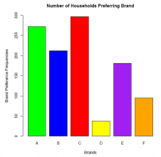
We have listed the arguments vertically (for the barplot() function), one per line, for the sake of minimizing clutter and improving visual clarity. In practice, however, there is no need to do so, and we can just as easily write the entire function (with its six arguments) on one line.

Answer:

#Comment1. Use the table() function to produce a frequency
#distribution and read the result into object named fd.
fd <- table(E2_1)
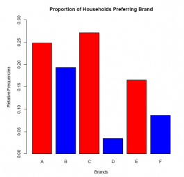
#Comment2. Create relative frequencies and assign to object rf.
rf <- fd / sum(fd)
#Comment3. Use the barplot() function to produce bar graph.
barplot(rf,

col = c('red', 'blue', 'red', 'blue', 'red', 'blue'),
ylim = c(0, 0.30),
xlab ='Brands',
ylab ='Relative Frequencies',
main = 'Proportion of Households Preferring Brand')

Answer:

#Comment1. Use the table() function to produce a frequency
#distribution and read the result into object named fd.
fd <- table(E2_1)
#Comment2. Create relative frequencies and assign to object rf.
rf <- fd / sum(fd)
#Comment3. Use the dotchart() function to create a dot plot.
dotchart(sort(rf),

xlab ='Relative Frequencies Brand is Preferred',
main ='Relative Frequencies by Brand',
pch = 20,
col ='blue')

## Warning in dotchart(sort(rf), xlab = "Relative Frequencies Brand is Preferred", : 'x' is neither a vector nor a matrix: using as.numeric(x)

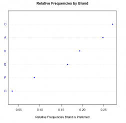
Note: it is necessary to sort the relative frequency data if we want the points in the dot plot to run in sequential order from the lower-left to the upper-right. This is done by nesting the sort() function as an argument in the dotchart() function. If we omit the sort() function, and include only the object name (in this case rf), the points in the plot are ordered alphabetically by default.

Note: This routine provides a warning message that we are free to ignore because the dotchart() function executes successfully and produces the dot plot image.

Answer:

#Comment1. Use the c() function and read result into object E2_2.
E2_2 <- c(24, 29, 34, 29, 37, 26, 30, 34, 30, 11, 12, 14, 18, 38, 17, 13, 16, 12, 33, 35, 35, 29, 28, 26, 25, 34, 11, 16, 19, 11, 13, 36, 12, 12, 12, 26, 36, 16, 26, 22, 15, 29, 38, 34, 30)
#Comment2. Read data into the object brks.
brks <- c(10, 14.99, 19.99, 24.99, 29.99, 34.99, 39.99)
#Comment3. Use cut() function to assign values in E2_2 to categories
#defined by brks: (10,15], (15,20], (20,25], (25,30], (30,35],

#(35,40]; read this result into object named categ.
categ <- cut(E2_2, brks)
#Comment4. Use table() function to produce frequency distribution of
#data items in categ; read the result into object fd.
fd <- table(categ)
#Comment5. Examine contents of fd.
fd
## categ
##  (10,15]  (15,20]  (20,25]  (25,30]  (30,35]  (35,40]
##    11            7         2            10         8            7

Thus, 11 values fall in the first category (between 10 and 15), 7 in the second (from 15 to 20), 2 in the third, 10 in the fourth, 8 in the fifth, and 7 in the sixth.

Answer:

#Comment1. Create relative frequencies by dividing each element in
#fd by total number of data values; read result into object rf.
rf <- fd / sum(fd)
#Comment2. Examine contents of rf.
rf
## categ
##   (10,15]                (15,20]         (20,25]              (25,30]          (30,35]           (35,40]
##  0.24444444   0.15555556   0.04444444   0.22222222    0.17777778    0.15555556

Thus, 0.24 of observations fall in the first class, 0.16 fall in the second, 0.04 in the third, 0.22 in the fourth, 0.18 in the fifth, and 0.16 fall in the sixth class.

Answer:

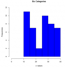
#Comment. Use the hist() function to create a histogram
hist(E2_2,

breaks = c(9.99, 14.99, 19.99, 24.99, 29.99, 34.99, 39.99),

xlim = c(0, 45),

ylim = c(0, 12),

xlab =  'x-values',

ylab = 'Frequencies',

main =' Six Categories',

col = 'blue')

Answer:

#Comment1. Import the a data set into the object E2_3.
E2_3 <- a
#Comment2. Use summary() function to find the smallest and largest
#values as well as the mean and median of E2_3.
summary(E2_3)
##               var1
##  Min.        :   6.721
##  1st Qu.    :28.336
##  Median   :51.181
##  Mean      :50.010
##  3rd Qu.   :70.345
##  Max.       :97.739

Since the smallest value is 6.721 and the largest is 97.74, we need to partition the histogram into ve categories roughly (97.74–6.721/5) = 91.02=5 ≈ 20 units wide. Since the median and mean are almost equal, the data may be normally (or at least symmetically) distributed.

Answer:

#Comment1. Use the names() function to determine the variable name.
names(E2_3)
## [1] "var1"
#Comment2. Read data into the object brks.
brks <- c(0, 20, 40, 60, 80, 100)
#Comment3. Use the cut() function to assign values in E2_3 to
#categories defined by brks: (0,20], (20,40], (40,60], (60,80],
#(80,100]; read this result into object named categ.
categ <- cut(E2_3$var1, brks)
#Comment4. Use table() function to produce frequency distribution of
#data items in categ and read result into object fd.
fd <- table(categ)
#Comment5. Examine contents of fd.
fd
## categ
##  (0,20]  (20,40]  (40,60]  (60,80]  (80,100]
##  18         68           30         67          16
Thus, there are 18 values falling in the first category, 68 in the second, 30 in the third, 67 in the fourth, and 16 in the fifth. It appears that a frequency distribution with 5 classes spreads out and classifes the 199 data items pretty well. Interestingly, although the summary statistics seem to suggest that the distribution might be somewhat normally distributed—since the mean and median are nearly equal—
the frequency distribution makes clear that the data are not distributed normally, but bimodally.

Answer:

#Comment1. Create relative frequencies by dividing fd by total
#number of data values. Read result into object named rf.
rf <- fd / sum(fd)
#Comment2. Request the relative frequency distribution.
rf
## categ
##  (0,20]                  (20,40]        (40,60]            (60,80]       (80,100]
## 0.09045226   0.34170854   0.15075377   0.33668342   0.08040201
Thus, 0.09 (of counts) fall in the first category, 0.34 fall in the second, 0.15 in the third, 0.34 in the fourth, and 0.08 in the fifth.

Answer:

#Comment. Use the hist() function to create a histogram.
hist(E2_3$var1,

breaks = c(0, 20, 40, 60, 80, 100),
col = 'purple',
ylim = c(0, 80),
xlab = 'x values',
ylab = 'Frequencies',
main = 'Five Categories')

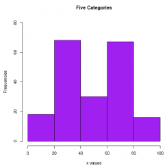
The histogram makes clear that even though the central tendency of the distribution is about 50 (according to the mean and the median), the data are indeed bimodal, not normal.

Answer:

#Comment. Use function hist() to create a histogram.
hist(E2_3$var1,

breaks = 10,
col = 'green',
ylim = c(0, 40),
xlab = ' x values',
ylab = 'Frequencies' ,
main = '10 Categories')

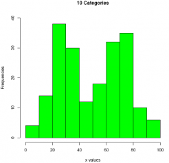
(Note that instead of defining the classes using breaks=c() as we did in the previous exercise, we can also use breaks=10. See the second argument of the hist ()function above.)

On closer inspection, it appears that using 10 categories rather than 5 offers no further resolution to the distribution of the data values. Even so, it is sometimes advantageous to break up the data into more (but narrower) categories because patterns that were not discernable with a smaller number of categories may be revealed when the data are spread out into more categories.

The next three exercises provide a bit of practice writing basic R code for the purpose of creating an image and interpreting its meaning. The three data sets are plot1, plot2, and plot3, and can be found on the companion website.

Answer:

#Comment1. Use the head(,3) function to identify the variable
#names and first 3 data records.
head(plot1, 3)
##         x    y
##    1   -3  4
##    2   -3  3
##    3   -2  3

#Comment2. Use the plot() function to create a scatter diagram
#of the two variables.
plot(plot1$x, plot1$y,

pch = 21,
col = "blue",
xlab = "x",
ylab = "y")

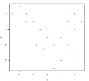
The scatter plot probably works best of all because it provides a picture of the association between two variables very clearly. In this case, the relationship between the two variables x and y is not linear but more parabolic.

Answer:

#Comment1. Use the head(,3) function to identify the variable
#names and first 3 data records.
head(plot2, 3)
##          x    y
##   1   -23  24
##   2   -33  50
##   3   1 9

#Comment2. Use the plot() function to create a scatter diagram
#of the two variables.
plot(plot2$x, plot2$y,

pch = 23,
col = "red",
xlab = "x",
ylab = "y")

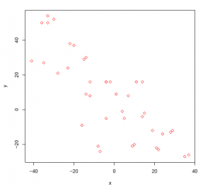
The two variables x and y appear to be negatively (and linearly) related.

Answer:

#Comment1. Use the head(,3) function to identify the variable
#names and first 3 data records.
head(plot3, 3)
##         x   y
##   1   -3  -4
##   2   15  9
##   3   23  21
#Comment2. Use the plot() function to create a scatter diagram
#of the two variables.

plot(plot3$x, plot3$y,

pch = 25,
col = "purple",
xlab = "x",
ylab = "y")

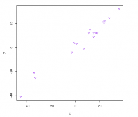
The variables x and y seem to be positively (and linearly) related.

The following exercises use the Cars93 data set that includes information on 93 makes and models of passenger vehicles on sale in the US in 1993. Since Cars93 must be downloaded from the MASS package, be sure to follow the directions provided at the beginning of the Chapter 2 end-of-chapter exercises in the book.

#Comment. Load the MASS package (contains the Cars93 data set).
library(MASS)
##
## Attaching package: 'MASS'
## The following object is masked from 'package:introstats':
##
## housing

Answer:

#Comment1. Read Cars93 data set into the object E2_4.
E2_4 <- Cars93
#Comment2. Use head() to display the 7 rows and 7 columns of Cars93.
head(E2_4[1 : 7], 7)
##       Manufacturer    Model   Type   Min.Price          Price   Max.Price    MPG.city
##    1        Acura        Integra   Small        12.9         15.9         18.8              25
##    2        Acura      Legend  Midsize       29.2         33.9         38.7              18
##    3       Audi                90   Compact     25.9         29.1         32.3              20
##    4       Audi              100   Midsize      30.8          37.7         44.6              19
##    5      BMW             535i   Midsize      23.7          30.0         36.2               22
##    6      Buick        Century Midsize       14.2          15.7        17.3               22
##   7       Buick       LeSabre Large          19.9           20.8       21.7               19
#Comment3. Use the table() function to produce a frequency
#distribution of Type; read the result into the object named fd.
fd <- table(E2_4$Type)
#Comment4. Examine the contents of fd.
fd
##
## Compact Large Midsize Small Sporty Van
## 16 11 22 21 14 9
As the frequency distribution of Type indicates, the 93 vehicles are distributed across 6 vehicle types: 22 vehicles are midsize, 21 are small, 16 are compact, 14 are sporty, 11 are large, and 9 are vans.

Answer:

#Comment1. Divide frequency distribution by number of observations.
#Assign the result to the object named rfd.
rfd <- fd / nrow(E2_4)
#Comment2. To examine the contents of rfd.
rfd

##
##  Compact           Large          Midsize             Small        Sporty             Van
##  0.17204301  0.11827957  0.23655914  0.22580645   0.15053763  0.09677419
#Comment3. Check to make sure the proportions sum to 1.
sum(rfd)
## [1] 1
The proportion of large passenger vehicles in the Cars93 data set is almost 0.12 (0.11828), or roughly 12%. When added up, the proportions sum to one.

Answer:

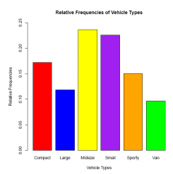
#Comment. Use the barplot() function to provide the bar graph.

barplot(rfd,

col = c('red','blue','yellow','purple','orange','green'),

xlab ='Vehicle Types',

ylab ='Relative Frequencies',

main ='Relative Frequencies of Vehicle Types,

ylim = c(0, 0.25))

Answer:

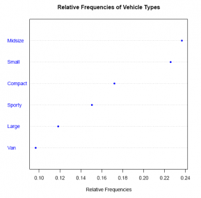
#Comment. Use the dotchart() function to create a dot plot

dotchart(sort(rfd),

main ='Relative Frequencies of Vehicle Types',

xlab ='Relative Frequencies',

pch = 20,

col ='blue')

## Warning in dotchart(sort(rfd), main = "Relative Frequencies of Vehicle
Types", : 'x' is neither a vector nor a matrix: using as.numeric(x)

Answer:

#Comment1. Read data into the object brks.

brks <- c(0, 10, 20, 30, 40, 50, 60, 70, 80)

#Comment2. Use the cut() function to assign values in E2_4 to
#categories defined by brks: (0,10], (10,20], (20,30], (30,40],
#(40,50], (50,60], (60,70],and (70,80]; read this result into
#object named categ.

categ <- cut(E2_4$Max.Price, brks)

#Comment3. Use the table() function to make frequency distribution
#of data items in categ. Read the result into object named fd.

fd <- table(categ)

#Comment4. Examine the contents of fd.

fd

## categ
##    (0,10]     (10,20]    (20,30]    (30,40]    (40,50]    (50,60]   (60,70]   (70,80]
##       8            39           30            11             3              1             0           1

The frequency distribution indicates that only 5 vehicles have prices above $40, 000; 8 have prices at $10, 000 or below. Most vehicles, 69 of them, are priced in the $10, 000 to $30, 000 range.

Answer:

#Comment1. Create relative frequencies by dividing fd by total

#number of data values. Read the result into object named rfd.

rfd <- fd / sum(fd)

#Comment2. Examine contents of rfd.

rfd

## categ

##    (0,10]                  (10,20]       (20,30]                  (30,40]            (40,50]        (50,60]

##    0.08602151     0.41935484    0.32258065   0.11827957   0.03225806   0.01075269

##    (60,70]                 (70,80]

##   0.00000000       0.01075269

#Comment3. Check to make sure the relative frequencies sum to 1.

sum(rfd)

## [1] 1

From the relative frequencies, it is clear that nearly 75% of the maximum prices for all passenger vehicles in the Cars93 data set fall in the $10, 000 to $30, 000 range; just over 17% are priced over $30, 000 while less than 9% come in at under $10, 000. All frequencies sum to one.

Answer:

#Comment. Use the hist() function with breaks=8.

hist(E2_4$Max.Price,

breaks = 8,

xlab ='Maximum Price of Passenger Vehicles (in $000)',

main ='Frequencies of Prices,

col = c('red','pink','blue,'yellow','purple','orange','grey','green'))

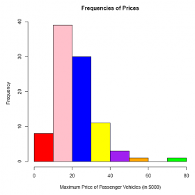
The frequency distribution as depicted by the histogram appears to be slightly skewed (from the normal distribution) to the right. Two outliers appear, one at $80, 000 (the Mercedes Benz 300E) and one at $50, 400 (the In niti Q45).

Answer:

#Comment1. Use the table() function to create a cross-tabulation

#table of Type and Origin. Name the resulting object crosstab.

crosstab <- table(E2_4$Type, E2_4$Origin)

#Comment2. Exam the contents of crosstab.

crosstab

##
##               USA non-USA
##   Compact    7        9
##   Large       11        0
##   Midsize     10     12
##   Small          7     14
##   Sporty        8       6
##    Van           5       4

As the cross-tabulation table makes clear, all of the large vehicles are of US-origin.

#Comment1. Use the table() function to create a cross-tabulation
#table of Man.trans.avail and Origin. Read the result into the
#object named crosstab.

crosstab <- table(E2_4$Man.trans.avail, E2_4$Origin)

#Comment2. Examine the contents of crosstab.

crosstab

##
##             USA non-USA
##    No         26        6
##    Yes       22       39

#Comment1. Use the rowSums() function to get totals across rows of
#crosstab; name the result Totals.

Totals <- rowSums(crosstab)

#Comment2. Use the cbind() function to bind column Totals to
#crosstab; recycle the result into the object crosstab.

crosstab <- cbind(crosstab, Totals)

#Comment3. Use the colSums() function to get totals down columns of
#crosstab; name the result Totals.

Totals <- colSums(crosstab)

#Comment4. Use the rbind() function to bind row Totals to crosstab;
#recycle the result into the object crosstab.

crosstab <- rbind(crosstab, Totals)

#Comment5. Examine the contents of crosstab.

crosstab

##           USA non-USA Totals
##   No         26          6      32
##   Yes       22          39    61
##   Totals    48          45   93

The cross-tabulation table makes clear that a much larger percentage of vehicles offering buyers the option of a manual transmission are of non-US origin, 87% (or 39 of 45) to only 46% (or 22 of 48) for vehicles of US origin.

Answer:

#Comment1. Read data into the object brks.

brks <- c(0, 2, 4, 6)

#Comment2. Use the cut() function to assign values in E2_4
#(EngineSize) to categories defined by brks: (0,2], (2,4],
#and (4,6]; read this result into object named displacement.

displacement <- cut(E2_4$EngineSize, brks)

#Comment3. Read data into the object brks.

brks <- c(0, 20, 40, 60, 80)

#Comment4. Use the cut() function to assign values in E2_4
#(Max.Price) to categories defined by brks: (0,20], (20,40],
#(40,60], and (60,80]; read this result into object named price.

price <- cut(E2_4$Max.Price, brks)

#Comment5. Use the table() function to create a cross-tabulation
#table of EngineSize and Max.Price. Name the table crosstab.

crosstab <- table(displacement, price)

#Comment6. Exam the contents of crosstab.

crosstab
## price
##   displacement   (0,20]    (20,40]    (40,60]    (60,80]
##                (0,2]      27             2             0            0
##                (2,4]      18           35             1            1
##                (4,6]        2            4              3            0

Answer:

#Comment1. Apply rownames() function to crosstab, incorporating
#the new row names: 1 to 2 liters, 2 to 4 liters, 4 to 6 liters.

rownames(crosstab) <- c('1 to 2 liters','2 to 4 liters','4 to 6 liters')

#Comment2. Apply colnames() function to crosstab, incorporating
#the new column names: Economy, Mid-Price, Higher-Price, Luxury.

colnames(crosstab) <- c('Economy','Mid-Price','Higher-Price','Luxury')

#Comment3. Examine contents of crosstab.

crosstab

##   price
##    displacement      Economy    Mid-Price   Higher-Price   Luxury
##    1 to 2 liters                27                 2                      0           0
##     2 to 4 liters               18               35                      1           1
##     4 to 6 liters                 2                4                       3           0

Answer:

#Comment1. Use the rowSums() function to get totals across rows of
#crosstab; name the result Totals.

Totals <- rowSums(crosstab)

#Comment2. Use the cbind() function to bind column Totals to crosstab;
#recycle the result into the object crosstab.

crosstab <- cbind(crosstab, Totals)

#Comment3. Use the colSums() function to get totals down columns of
#crosstab; name the result Totals.

Totals <- colSums(crosstab)

#Comment4. Use the rbind() function to bind row Totals to crosstab;
#recycle the result into the object crosstab.

crosstab <- rbind(crosstab, Totals)

crosstab <- rbind(crosstab, Totals)
#Comment5. Examine the contents of crosstab.

crosstab

crosstab
##                                  Economy        Mid-Price     Higher-Price   Luxury    Totals
##       1 to 2 liters            27                     2                          0             0          29
##       2 to 4 liters            18                    35                         1             1          55
##       4 to 6 liters              2                      4                          3             0           9
##       Totals                     47                     41                        4             1          93

Answer:

#Comment. Use the plot() function with Max.Price on the horizontal
#axis, EngineSize on the vertical.

plot(E2_4$Max.Price, E2_4$EngineSize,

main ='A Scatter Diagram Relating Engine Size and Price',
pch = 23,
col ='orange',
ylab ='Engine Displacement in Liters',
xlab ='Vehicle Price')

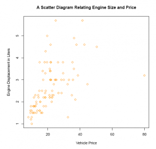
In general, there appears to be a positive relationship between engine size and price: engine size is (roughly) positively related to vehicle price.

Answer:

#Comment. Use the plot() function with EngineSize on the horizontal
#axis, Horsepower on the vertical.

plot(E2_4$EngineSize, E2_4$Horsepower,

main ='A Scatter Diagram Relating Engine Size and Horsepower',
xlab ='Engine Displacement in Liters',
ylab ='Maximum Horsepower',
pch = 19,
col ='blue')

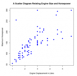
As expected, these two variables are positively and linearly related: in general, the larger the engine, the greater the horsepower.

Answer:

#Comment. Use plot() function with EngineSize on the horizontal
#axis, MPG.highway on the vertical.

plot(E2_4$EngineSize, E2_4$MPG.highway,

main ='A Scatter Diagram Relating Engine Size and Miles Per US Gallon',
xlab ='Engine Displacement in Liters',
ylab ='Highway Miles Per US Gallon',
pch = 24,
col ='red')

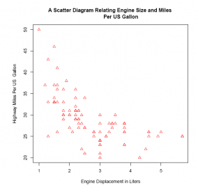
Unsurprisingly, the two variables are negatively (and somewhat linearly) related: in general, the larger the engine size, the lower the gasoline mileage.

Answer:

#Comment. Use the plot() function with Max.Price on the horizontal
#axis, RPM on the vertical.

plot(E2_4$Max.Price, E2_4$RPM,

main ='A Scatter Diagram Relating Vehicle Price and Revs per Minute',
ylab ='Revs per Minute at Maximum Horsepower',
xlab ='Vehicle Price',
pch = 20,
col ='purple')

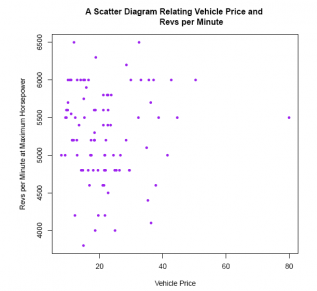
Since there is no reason to suspect that these two particular variables are related, either positively or negatively, we are not surprised to see this cloud of data points.