Statistics with R
Student Resources
Chapter 13: Multiple Regression
##
## Attaching package: 'MASS'
## The following object is masked from 'package:introstats':
##
## housing
#Comment1. Import Cars93 into the object named E13_1.
E13_1 <- Cars93
#Comment2. Use nrow() function to find number of observations.
nrow(E13_1)
## [1] 93
#Comment3. Use names() function to list variable names.
names(E13_1)
## [1] "Manufacturer" "Model" "Type"
## [4] "Min.Price" "Price" "Max.Price"
## [7] "MPG.city" "MPG.highway" "AirBags"
## [10] "DriveTrain" "Cylinders" "EngineSize"
## [13] "Horsepower" "RPM" "Rev.per.mile"
## [16] "Man.trans.avail" "Fuel.tank.capacity" "Passengers"
## [19] "Length" "Wheelbase" "Width"
## [22] "Turn.circle" "Rear.seat.room" "Luggage.room"
## [25] "Weight" "Origin" "Make" #Comment4. Use the table() function to find the distribution
#of vehicle types.
table(E13_1$Type)
##
## Compact Large Midsize Small Sporty Van
## 16 11 22 21 14 9
Answer: There are 93 observations in Cars93 (now E13_1); the 27 variable names are listed under Comment 3. As to vehicle Type, the frequency distribution is provided under Comment 4.
2. Subset the E13_1 data to exclude all observations for which Type is either Sporty or Van; import the result into the object E13_2. How many observations are included in E13_2? Does the frequency distribution for the Type variable in E13_2 show that the Sporty and Van observations have been excluded?
#Comment1. Set indexing [ ] to drop all observations that include
#either Sporty or Van. (Note that the exclamation point ! must be
#used before each condition. Thus, we direct the code to return
#data that include all variables EXCEPT those for which Type is
#either Sporty or Van.) Import into object E13_2.
E13_2 <- E13_1[!(E13_1$Type=="Sporty") & !(E13_1$Type=="Van"), ]
#Comment2. Use nrow() function to find number of observations in
#the new object E13_2.
nrow(E13_2)
## [1] 70
#Comment3. Use the table() function to find the distribution of
#vehicle types included in object E13_2.
table(E13_2$Type)
##
## Compact Large Midsize Small Sporty Van
## 16 11 22 21 0 0
Answer: Yes, the object E13_2 no longer includes any sporty vehicles or vans. The number of observations in E13_2 has fallen from 93 to 70.
3. For a little more practice at “shaping” our data before the actual analysis, subset E13_2 (one more time) to exclude all variables except for MPG.city, Weight, and Passengers and import into an object named E13_3. List the variable names. How many observations are there?.
#Comment1. Set indexing [ ] to drop all variables except
#MPG.city, Weight, and Passengers. Import into E13_3.
E13_3 <- E13_2[, c("MPG.city", "Weight","Passengers")]
#Comment2. Use names() function to list variable names.
names(E13_3)
## [1] "MPG.city" "Weight" "Passengers"
#Comment3. Use nrow() function to find number of observations in
#the new object E13_3.
nrow(E13_3)
## [1] 70
#Comment4. Use summary() and table() functions to find the basic
#descriptive statistics for variables.
summary(E13_3$MPG.city)
## Min. 1st Qu. Median Mean 3rd Qu. Max.
## 16.00 19.00 22.00 23.17 25.00 46.00
summary(E13_3$Weight)
## Min. 1st Qu. Median Mean 3rd Qu. Max.
## 1695 2534 3008 3010 3495 4105
table(E13_3$Passengers)
##
## 4 5 6
## 11 41 18
Answer: There are 70 observations across the 3 variables MPG.city, Weight, and Passengers in the object E13_3. The basic descriptive statistics are provided under Comments 4 and 5. Note: there is no compelling reason why we have to drop all variables as we have here. The statistical part of our analysis can proceed with or without them just fine. For this exercise, we have done so only because it provides the opportunity to get additional practice subsetting data and because we have tidied up the data (good housekeeping). The data now include only those observations and variables we are most interested in.
4. In an attempt to build a regression model with more explanatory and predictive power than what we were able to achieve in the Chapter 12 Exercises, we now exchange the independent variable EngineSize for two other variables Weight and Passengers. (In this exercise, the dependent variable is still MPG.city.) As a first step, use the pairs() function to verify that each independent variable is linearly related to the dependent variable but not strongly related to one another. Comment.
#Comment. Use the pairs() function to create a scatterplot of
#all variables, taken pairwise. Set lower.panel=NULL to suppress
#producing plots in the lower diagonal (redundant).
pairs(E13_3, pch = 19, lower.panel = NULL)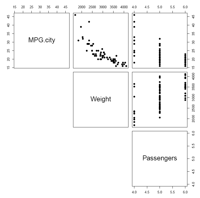
.
Answer: A peculiarity that the scatterplots reveal is the odd configuration of points in the two righthand plots, which depict the relationship between the independent variable Passengers and the other two variables, MPG.city and Weight. In particular, the points seem stacked on top of one another for three values of Passengers. When we consider what the variable Passengers measures—a vehicle’s passenger capacity (persons)—the explanation is clear: the data include only those vehicles that can accommodate 4, 5, or 6 passengers. (Remember that we have dropped those observations that include sports cars and vans, vehicles that presumably accommodate different numbers of passengers.) Even so, we can see that the relationship between Passengers and MPG.city is generally negative; that is, vehicles that can accommodate more passengers tend to have poorer city mileage. Between Passengers and Weight the relationship is generally positive—vehicles that can accommodate more passengers are heavier—an association that is evidence of some multicollinearity. Finally, the relationship between Weight and MPG.city appears to be both negative and relatively linear.
5. Mention has been made (in the preceding exercise) about the possibility of multi-collinearity between two of the variables, Passengers and Weight. Can you think of any other way to explore whether this might be a problem?
#Comment. Use the cor() function to find the correlation.
cor(E13_3$Passengers, E13_3$Weight)
## [1] 0.5732935
Answer: While a correlation of r = 0:5732935 is a clear and unambiguous indicator of the presence of multicollinearity between these two independent variables, it is not so severe that we cannot conduct the analysis at all. In fact, some authorities report the rule-of-thumb they use as this: if |r| > 0:70—that is, if r > 0:70 or r < –0:70—we would probably not introduce both variables. Since r = 0:5732935 does not fall in that range, we include both independent variables in this analysis.
6. Make and inspect a residual plot. Does the pattern reveal anything that might call into question the appropriateness of this methodology when applied to this data?
#Comment1. Use the lm() function to create the model object named
#mr1 (the first multiple regression model).
mr1 <- lm(MPG.city ~ Weight + Passengers, data = E13_3)
#Comment2. Use the plot() function to create a residual plot.
#Note that resid(mr1) must be included as an argument.
plot(fitted(mr1), resid(mr1),
abline(h = 0),
pch = 19,
xlab = 'Predicted Value of y' ,
ylab = 'Residuals' )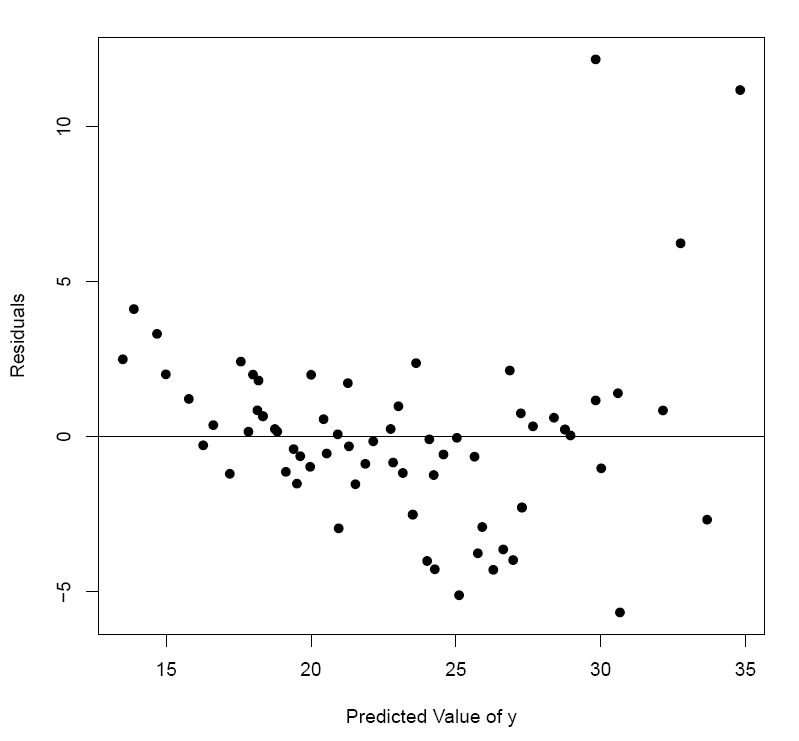
Answer: This is a good place to reprise the basic assumptions about the model of the relationship between y and the independent variables x1, x2,..., xk. The reason why we revisit the discussion here is that an analysis of the residuals is an important step that is sometimes overlooked or even misunderstood by analysts. Recall that the residuals or the error terms are defined as ![]()
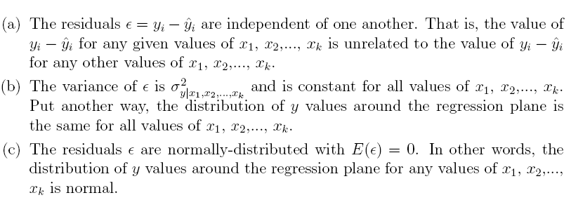
A good way to confirm whether a set of variables conforms to the assumptions underlying the correct usage of regression analysis is to create and inspect a plot of theresiduals ![]() against the independent variable x . However, one difference between what we did in the case of simple linear regression and how we go about it for multiple regression is that we do not usually plot the residuals against the independent variable for the reason that we now have more than one of them. (In fact,
against the independent variable x . However, one difference between what we did in the case of simple linear regression and how we go about it for multiple regression is that we do not usually plot the residuals against the independent variable for the reason that we now have more than one of them. (In fact,
the residuals are sometimes plotted against the individual independent variables, one by one, but we do not do that here.) In view of this, we can instead plot the residuals against the predicted value of the dependent variable ŷ.
A cursory inspection of the residual plot reveals that the above 3 assumptions underlying the correct application of a regression model to any set of data are not very well satisfied. For one thing, the variance of s is not constant across the range of ŷ values. For another, the residuals s do not appear to be normally-distributed.
For these reasons, we must be cautious in not only how we apply the regression (when, for example, for purposes of prediction) but also in our interpretation of it. We can still conduct the regression analysis on the E13_3 data, as we intend to do in the next exercises, but we must bear in mind the reality that (like so many sets of data) the assumptions behind the appropriate application of regression analysis are poorly met.
7. As part of making the residual plot in the preceding exercise, we used the lm() function to create mr1, the model object that includes all the important information associated with the regression problem, including the estimated regression equation itself. What is the estimated regression equation?
mr1
##
## Call:
## lm(formula = MPG.city ~ Weight + Passengers, data = E13_3)
##
## Coefficients:
## (Intercept) Weight Passengers
## 53.644618 -0.007617 -1.479297
Answer: The estimated regression equation is ŷ = b0 + b1x1 + b2x2 = 53:644618 – 0:007617x1 – 1:479297x2 where ŷ is the predicted dependent variable; as to the independent variables, x1 is Weight and x2 is Passengers.
8. Find the 70 percent confidence interval estimates of the regression coefficients b1 and b2. Describe what these confidence intervals mean.
#Comment. Use the confint(, level =) function to find the
#confidence interval estimates of the regression coefficients.
confint(mr1, level = 0.70)
## 15 % 85 %
## (Intercept) 50.594506526 56.69472945
## Weight -0.008404125 -0.00683022
## Passengers -2.200999813 -0.75759321
Answer: There is a 70% probability that the regression coefficient b1 falls in the interval from –0.008404125 to –0.00683022, and the regression coefficient b2 falls in the interval from –2.200999813 to –0.75759321.
9. What does the estimated regression equation tell us?
Answer: At least for this data (which excludes sports cars and vans), we can say that a 1 pound change in vehicle Weight is associated with a 0.007617 change in MPG.city if we hold the Passenger vehicle capacity constant. Moreover, a 1 Passenger change in vehicle capacity is associated with a 1.479297 change in MPG.city if we hold the vehicle Weight constant. Since the partial regression coefficients have a negative sign, we know that (1) MPG.city and Weight are negatively associated: as Weight
increases (decreases), the MPG.city decreases (increases); and (2) MPG.city and Passengers are negatively associated: as Passengers increases (decreases), the MPG.city decreases (increases). As in the case with simple linear regression, the intercept term b0 = 53.644618 is not meaningful. We retain it in the regression equation itself, however, for reasons of prediction.
10. What is the strength of association between the independent variables, Weight and Passenger, and MPG.city, the dependent variable? Find the coefficient of determination r2 using the following expression (do not use the summary() function to unpack the regression statistics; we will use it later). This exercise provides another opportunity to sharpen your coding skills.

#Comment1. Find the total sum of squares, ss_y.
ss_y <- sum((E13_3$MPG.city - mean(E13_3$MPG.city)) ^ 2)
#Comment2. Find the residual sum of squares, ss_res.
ss_res <- sum((resid(mr1)) ^ 2)
#Comment3. Find the coefficient of determination. Import the
#result into the object named r_square.
r_square <- (ss_y - ss_res) / ss_y
#Comment4. What is the value of r-square?
r_square
## [1] 0.7453017
Answer: The coefficient of determination, r2 = 0.7453017.
11. What does the coefficient of determination r2 reveal about the regression model?
Answer: We interpret r2 = 0.7453017 in the following way: approximately 74.53% of the variation in the dependent variable ŷ (MPG.city) can be be accounted for (or explained) by the variation in the two independent variables, x1 (Weight) and x2 (Passengers). We also know that roughly 25.47% of the variation in ŷ remains unexplained or unaccounted for.
12. What is the adjusted coefficient of determination?
Answer: adjusted-r2 = 0.7377.
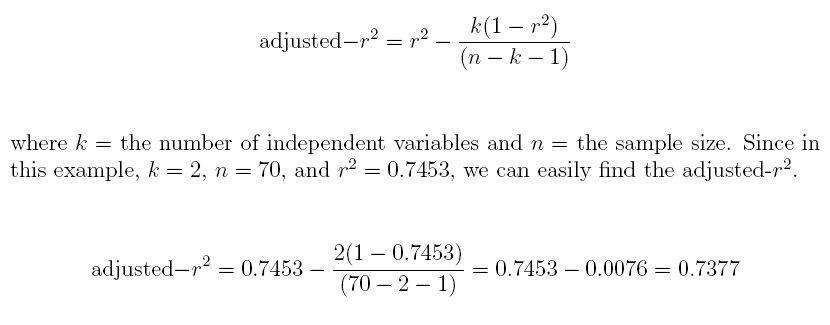
adj_r_square <- r_square - (2 * (1 - r_square)) / (70 - 2 - 1)
adj_r_square
## [1] 0.7376987
13. What is the F statistic for the overall regression model?
Answer: F = 98.02815
where

#Comment1. Find the numerator of the numerator.
ss_reg <- sum((fitted(mr1) - mean(E13_3$MPG.city)) ^ 2)
#Comment2. Find the numerator of the F statistic.
F_numer <- ss_reg / 2
#Comment3. What is the numerator of the F statistic?
F_numer
## [1] 889.1236
#Comment4. Find the numerator of the denominator.
ss_res <- sum((resid(mr1)) ^ 2)
#Comment5. Find the denominator of the F statistic.
F_denom <- ss_res / (70 - 2 - 1)
#Comment6. What is the denominator of the F statistic?
F_denom
## [1] 9.070084
#Comment7. The ratio of F_numer to F_denom is the F statistic.
F <- F_numer / F_denom
#Comment8. What is the F statistic?
F
## [1] 98.02815
14. For this regression equation, complete the missing entries in the ANOVA table.
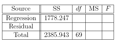
Answer: The missing entries are the bolded numbers in the following table.

#Comment1. Calculations for the first row of missing values.
ss_reg <- sum((fitted(mr1) - mean(E13_3$MPG.city)) ^ 2)
ss_reg
## [1] 1778.247
ms_reg <- ss_reg / 2
ms_reg
## [1] 889.1236
#Comment2. Calculations for the second row of missing values.
ss_res <- sum((resid(mr1)) ^ 2)
ss_res
## [1] 607.6957
ms_res <- ss_res/ (70 - 2 - 1)
ms_res
## [1] 9.070084
#Comment3. Calculation for the F statistic.
f <- ms_reg / ms_res
f
## [1] 98.02815
15. What is the p-value for F = 98.02815 for dfN = k = 2 and dfD = n – k –1 =70 – 2 –1 = 67?
![]()
options(scipen = 999)
pf(98.02815, 2, 67, lower.tail = FALSE)
## [1] 0.0000000000000000000126437
16. Complete the missing entries in this table, including the values of t as well as the associated p-values for the two regression coefficients.

Answer: The missing entries are the bolded numbers in the following table.

#p-value for bo
2 * pt(18.371, 68, lower.tail = FALSE)
## [1] 0.0000000000000000000000000004534737
#p-value for b1
2 * pt(-10.110, 68)
## [1] 0.000000000000003486782
#p-value for b2
2 * pt(-2.141, 68)
## [1] 0.03586164
17. Use the summary() extractor function to check our work. Remember to use the model object mr1 as the argument. Are the reported statistics in agreement with those worked out in the previous exercises?
#Comment1. Use options(scipen=999) to report extremely small values
#in standard (not scientific) notation.
options(scipen = 999)
#Comment2. Use the summary() function to extract
#the regression statistics.
summary(mr1)
##
## Call:
## lm(formula = MPG.city ~ Weight + Passengers, data = E13_3)
##
## Residuals:
## Min 1Q Median 3Q Max
## -5.6650 -1.2245 0.0043 0.9515 12.1729
##
## Coefficients:
## Estimate Std. Error t value Pr(>|t|)
## (Intercept) 53.6446180 2.9201150 18.371 < 0.0000000000000002 ***
## Weight -0.0076172 0.0007534 -10.110 0.00000000000000411 ***
## Passengers -1.4792965 0.6909441 -2.141 0.0359 *
## ---
## Signif. codes: 0 '***' 0.001 '**' 0.01 '*' 0.05 '.' 0.1 ' ' 1
##
## Residual standard error: 3.012 on 67 degrees of freedom
## Multiple R-squared: 0.7453,Adjusted R-squared: 0.7377
## F-statistic: 98.03 on 2 and 67 DF, p-value: < 0.00000000000000022
Answer: All the results arrived at using the summary() function confirm what
has been found in the preceding exercises: the estimated regression equation is ŷ = 53.6446180 – 0.0076172x1 – 1.4792965x2; the coefficient of determination is r2 = 0.7453; the adjusted-r2 = 0.7377; the F statistic is F = 98.03; and the F statistic has p-value=0.0000000000000000000126437.
We may safely ignore the slight disparity between the p-value reported here (found by executing the lm() function) and the p-value found by writing out the code in the previous exercise. For functions like lm(), the smallest floating point stored and printed by R is 2.2e-16 (a value with 15 zeros). This is why the last line of the printout above includes notation we have not seen before: p-value< 0:00000000000000022.
When an actual value includes more than 15 zeros, as our has in the preceding exercise—where p-value=0.0000000000000000000126437 includes 19 zeros—the lm() function simply reports p-value:< 0.00000000000000022. The only reason we mention this is because we might wonder why there is any di erence at all. Practically speaking, of course, there is no real diffierence in these values.
18. Use the estimated regression equation and the predict() function to nd the predicted values of MPG.city for the following values: for the first pair Weight=2000 and Passengers=6, for the second pair Weight=3000 and Passengers=5, and the third pair Weight=4000 and Passengers=4.
#Comment1. Use data.frame() to create a new object. Name the
#new object newvalues.
newvalues <- data.frame(Weight = c(2000, 3000, 4000), Passengers = c(6, 5, 4))
#Comment2. Examine the contents of the object named newvalues
#just to make sure it contains what we think it does.
newvalues
## Weight Passengers
## 1 2000 6
## 2 3000 5
## 3 4000 4
#Comment3. Use predict() function to provide the predicted values
#of miles per gallon for the new values of Weight and Passengers.
predict(mr1, newvalues)
## 1 2 3
## 29.53449 23.39662 17.25874
Answer: For the first pair Weight=2000 and Passengers=6, the predicted value ŷ is
29.53449 mpg; for the second pair Weight=3000 and Passengers=5, the predicted value ŷ is 23.39662; and for the third pair Weight=4000 and Passengers=4, the predicted value ŷ is 17.25874 mpg.
19. What are the predicted values of MPG.city that were used to calibrate the estimated regression equation ŷ = 53.6446180 – 0.0076172x1 – 1.4792965x2? Import those predicted values into an object named mileage_predicted and list the first and last three elements.
Answer: #Comment1. Use fitted(mr1) function to create the predicted
#values of the dependent variable. Import those values into
#the object named mileage_predicted.
mileage_predicted <- fitted(mr1)
#Comment2. Use the head(,3) and tail(,3) functions to list the
#first and final three values of predicted values.
head(mileage_predicted, 3)
## 1 2 3
## 25.64368 19.13100 20.54018
tail(mileage_predicted, 3)
## 90 92 93
## 23.51088 23.51088 21.53041
20. Add the mileage_predicted object (created in the preceding exercise) to E13_3, and name the resulting object E13_4. List the first and final four elements. Find the correlation of the actual and predicted variables; that is, the correlation of MPG.city and mileage predicted. Once you have the correlation, square it (i.e., raise it to the second power). Comment on the square of the correlation. What is it?
Answer: #Comment1. Use the cbind() function to bind the column
#mileage_predicted to E13_3. Name the new object E13_4.
E13_4 <- cbind(E13_3, mileage_predicted)
#Comment2. List the first and final four elements of E13_4.
head(E13_4, 4)
## MPG.city Weight Passengers mileage_predicted
## 1 25 2705 5 25.64368
## 2 18 3560 5 19.13100
## 3 20 3375 5 20.54018
## 4 19 3405 6 18.83237
tail(E13_4, 4)
## MPG.city Weight Passengers mileage_predicted
## 88 25 2240 4 30.66497
## 90 21 2985 5 23.51088
## 92 21 2985 5 23.51088
## 93 20 3245 5 21.53041
#Comment3. Find the correlation of the actual and predicted
#dependent variables. Store the result in an object named r.
r <- cor(E13_4$MPG.city, mileage_predicted)
#Comment4. Examine the contents of r.
r
## [1] 0.8633086
#Comment5. Square the value of r.
r^2
## [1] 0.7453017
The square of the correlation of the actual dependent variable and predicted dependent variable equals the coefficient of determination, r2.
21. Consider the following estimated regression equation: ŷ = 3536 + 1183x1 – 1208x2. Suppose the model is changed to reflect the deletion of x2 and the resulting estimated simple linear equation becomes ŷ = –10663 + 1386x1.
(a) How should we interpret the meaning of the coefficient on x1 in the estimated simple linear regression equation ŷ = –10663 + 1386x1?
Answer: A 1 unit change in the independent variable x1 is associated with an expected
change of 1,386 units in the dependent variable ŷ
(b) How should we interpret the meaning of the coefficient on x1 in the estimated multiple regression equation ŷ = 3536 + 1183x1 –1208x2?
Answer: A 1 unit change in the independent variable x1 is associated with an expected
change of 1,183 in the dependent variable ŷ if the other independent variable
x2 is held constant.
(c) Is there any evidence of multicollinearity? What might that evidence be?
Answer: There is some multicollinearity between x1 and x2 because the coefficient has changed from 1,386 to 1,183 with the introduction of x2 into the regression model. In the case when the independent variables are perfectly uncorrelated, the coeffcient is unchanged.
22. Interpret the results below and answer the following questions. Suppose we regress the dependent variable y on 4 independent variables x1, x2, x3, and x4. After running the regression on n = 16 observations, we have the following information: SSreg = 946.181 and SSres = 49.773. Please answer the following questions.
(a) What is the r2?
Answer: 0.95

(b) What is the adjusted–r2
Answer: 0.932

(c) What is the F statistic?
Answer: F = 52.277

(d) What is the p-value?
Answer: p-value=0.0000
= p(F > 52.277; 4, 11) =
pf(52.277, 4, 11, lower.tail = FALSE)
## [1] 0.0000004338219
(e) Is the overall regression model significant? Test at = 0:05 level of significance.
Answer: Yes, since p-value= 0:0000 <α = 0:05, we conclude that the estimated regression model is signicant.
23. Referring to the previous exercise, suppose we also have the following information about the partial regression coefficients.

(a) Is b1 significant at a = 0:05? What is its t value? What is its p-value?
Answer:
2 * pt(-0.2718, 11)
## [1] 0.7908094
(b) Is b2 significant at = 0:05? What is its t value? What is its p-value?
Answer: 
2 * pt(-2.5875, 11)
## [1] 0.0252505
(c) Is b3 significant at a = 0:05? What is its t value? What is its p-value?
Answer: Since t = 3:9340 and p-value= 0:002336 < a = 0:05, b3 is signicant.
2 * pt(3.9340, 11, lower.tail = FALSE)
## [1] 0.002335972
(d) Is b4 significant at a = 0:05? What is its t value? What is its p-value?
Answer: Since t = 1:8232 and p-value= 0:09554 > = 0:05, b4 is not significant.

2 * pt(1.8232, 11, lower.tail = FALSE)
## [1] 0.09553817
24. Consider the following estimated multiple regression equation:
![]()
(a) Complete the missing entries in this ANOVA table.

Answer: The answers to part (a) are the bolded numbers in the following table.

pf(21.1331, 3, 6, lower.tail = FALSE)
## [1] 0.001366979
(b) Complete the missing entries in this coefficients table.

Answer: The answers to part (b) are the bolded numbers in the following table.

#p-value for bo
2 * pt(-0.5737, 6)
## [1] 0.5870154
#p-value for b1
2 * pt(5.362, 6, lower.tail = FALSE)
## [1] 0.001724838
#p-value for b2
2 * pt(3.439, 6, lower.tail = FALSE)
## [1] 0.01381786
#p-value for b3
2 * pt(0.823, 6, lower.tail = FALSE)
## [1] 0.4419823
(c) What is the r2?
Answer: 0.914

(d) What is the adjusted-r2?
Answer: 0.871

25. This exercise uses the mtcars data set that is installed in R.
(a) Use the pairs() function to create a scatterplot matrix for 3 variables: mpg, cyl, and wt. What can we say about the relationships between these variables?
Answer: We can apply the pairs() function to a subset of mtcars which contains only variables mpg (column 1), cyl (column 2), and wt (column 6). We use the tail() function to identify the column position of each variable.
tail(mtcars, 2)
## mpg cyl disp hp drat wt qsec vs am gear carb
## Maserati Bora 15.0 8 301 335 3.54 3.57 14.6 0 1 5 8
## Volvo 142E 21.4 4 121 109 4.11 2.78 18.6 1 1 4 2
pairs(mtcars[, c(1, 2, 6)], pch = 19, lower.panel = NULL)
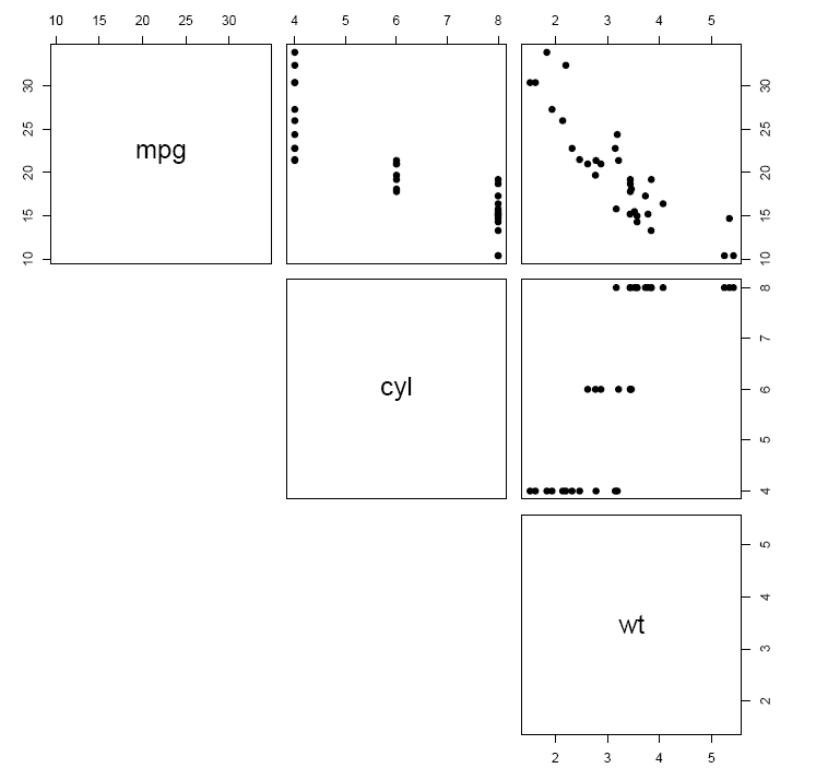
From the scatterplot, it is clear that mpg is negatively related to cyl and wt and that cyl is positively related to wt.
(b) Regress the dependent variable mpg on the variables cyl and wt. Write out the estimated regression equation.
reg_eq_mileage <- lm(mpg ~ cyl + wt, data = mtcars)
reg_eq_mileage
##
## Call:
## lm(formula = mpg ~ cyl + wt, data = mtcars)
##
## Coefficients:
## (Intercept) cyl wt
## 39.686 -1.508 -3.191
The estimated regression equation: ŷ = 39:69–1:51x1–3:19x2, where ŷ is thepredicted value of mpg, x1 is cyl, and x2 is wt. That the partial regression coefficients have a negative sign is unsurprising in view of the scatterplots above.
(c) Use the fitted function to create the predicted dependent variables for the values of cyl and wt in the original data set. Just to check that the predictions are correct, select 2 observations and work out the predicted value manually.
predicted <- fitted(reg_eq_mileage)
tail(predicted, 2)
## Maserati Bora Volvo 142E
## 16.23213 24.78418
Answer: From part (a), we see that for the Maserati Bora, cyl = 8 and wt = 3.57. Plugging these values into the estimated regression equation, we find that ŷ= 39.69 – 1.51x1 – 3.19x2 = 39.69 – 1.51(8) – 3.19(3.57) = 16.23. For the Volvo 142E, cyl = 4 and wt = 2.78, ŷ = 39.69–1.51(4)–3.19(2.78) = 24.78.
(d) Use the predict() function to create the predicted dependent variable for the following pairs of values of the independent variables: for the first pair cyl=4 and wt=5; for the second pair cyl=8 and wt=2
newvalues <- data.frame(cyl = c(4, 8), wt = c(5, 2))
predict(reg_eq_mileage, newvalues)
## 1 2
## 17.70022 21.24196
To check these predicted values, we simply plug (a) cyl = 4 and wt = 5 and
(b) cyl = 8 and wt = 2 into ŷ = 39.69–1.51x1–3.19x2 and find ŷ in each case:
ŷ = 39.69–1.51(4)–3.19(5) = 17.70 and ŷ = 39.69–1.51(8)–3.19(2) = 21.24.
