Chapter 12: Simple Linear Regression

1. This exercise provides further opportunity to find a set of data from an online source (such as www.infoplease.com), create a data frame from scratch (see the Chapter 1 Appendix, if necessary), and analyze it using some of the methods associated with simple linear regression. Look up and record the high and low intraday temperatures (either in degrees Celsius or Fahrenheit) for the following 14 cities from around the world: Auckland, Beijing, Cairo, Lagos, London, Mexico City, Mumbai, Paris, Rio de Janeiro, Sydney, Tokyo, Toronto, Vancouver, and Zurich. This information is easily found after brief search.

(a) Use c() to create three objects: one for each city name, one for the high temperature, and one for the low temperature. Data are recorded for December 19, 2016.

Answer:

city <- c('Auckland','Beijing','Cairo','Lagos','London','Mexico City', 'Mumbai','Paris','Rio de Janeiro','Sydney','Tokyo','Toronto','Vancouver','Zurich')
high <- c(71, 45, 65, 91, 46, 67, 88, 44, 92, 88, 57, 20, 42, 40)
low <- c(56, 23, 48, 76, 37, 45, 71, 35, 73, 65, 39, 15, 39, 29)

(b) Use data.frame() to create a data frame consisting of each city name and high and low temperatures. This results in an object with 14 observations on two variables. Display the results to check your work.

Answer:

WorldTemps <- data.frame(City = city, High = high, Low = low)
WorldTemps
##          City High   Low
## 1      Auckland    71         56
## 2              Beijing    45         23
## 3                Cairo    65         48
## 4   Lagos    91         76
## 5             London    46         37
## 6       Mexico City   67         45
## 7            Mumbai    88         71
## 8      Paris     44        35
## 9 Rio de Janeiro    92        73
## 10            Sydney   88        65
## 11              Tokyo    57        39
## 12           Toronto    20       15
## 13       Vancouver   42       39
## 14             Zurich    40       29

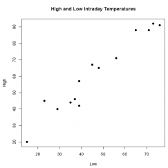
(c) Make a scatter plot of high against low temperatures. Create a main title, label each axis appropriately, and use pch = to specify how the points should appear. Does the pattern of points appear to confirm that the relationship between high and low temperatures is linear?

plot(WorldTemps$Low, WorldTemps$High, pch = 19, xlab = "Low", ylab = "High", main = "High and Low Intraday Temperatures")

Answer: The scatter plot makes clear that the relationship between high and low intraday temperatures is both positive and linear.

(d) Estimate and write out the regression equation: ŷ = b₀+b₁x. Let the high temperature be the dependent variable, and the low temperature, the independent variable.

reg_eq_temps <- lm(High ~ Low, data = WorldTemps)
reg_eq_temps
##
## Call:
## lm(formula = High ~ Low, data = WorldTemps)
##
## Coefficients:
## (Intercept) Low
## 7.763 1.148

Answer: The estimated regression equation is: ŷ = 7.76 + 1.15x.

(e) What is the value of r²?

summary(reg_eq_temps)

##
## Call:
## lm(formula = High ~ Low, data = WorldTemps)
##
## Residuals:
## Min 1Q Median 3Q Max
## -10.533 -3.991 -1.051 3.884 10.834
##
## Coefficients:
## Estimate Std. Error t value Pr(>|t|)
## (Intercept) 7.76313 4.27689 1.815 0.0946 .
## Low 1.14795 0.08546 13.433 1.36e-08 ***
## ---
## Signif. codes: 0 '***' ' 0.001'**' 0.01'*' 0.05 '.' 0.1' ' 1
##
## Residual standard error: 5.918 on 12 degrees of freedom
## Multiple R-squared: 0.9376,Adjusted R-squared: 0.9325
## F-statistic: 180.5 on 1 and 12 DF, p-value: 1.363e-08

Answer: The value of r² is 0.938, indicating that approximately 93:8% of variation in the dependent variable is explained by variation in the independent variable.

(f) What is the p-value? Is the estimate regession equation significant? Why or why not?

Answer: Since p-value = 0.0000000136 is far less than the usual values for (e.g., 0.05, 0.01), we would say that the estimated regression equation is significant.

2. A dependent variable y is regressed on an independent variable x; the sample size is n = 32.

(a) If SS_reg = 808.89 and SS_res = 317.16, what is r²?

Answer: 0.7183.

SS_y = SS_reg + SS_res = 808.89 + 317.16 = 1126.05

(b) If b₁ = –0.041215 and sb₁ = 0.004712, what is the value of the test statistic t?

Answer: t = –8.75.

Answer: p-value = 0.00000000093.

= 2(p(t <– 8.75, df = n–k–1)) = 2(p(t < –8.75, df = 30)) = 0.00000000093

2 * pt(-8.75, 30)

## [1] 9.313949e-10

(d) Is the estimated regression equation significant at the α = 0.01 level?

Answer: Yes, since the p-value = 0.00000000093 < α = 0.01, we conclude that the estimated regression equation is significant.

(e) If b₀ = 29.599855, write out the regression equation, ŷ = b₀ + b₁x.

Answer: ŷ = 29.599855 – 0.041215x

3. This exercise uses the mtcars data set that is installed in R. (Remember that to see all the installed data sets, simply enter data() at the R prompt in the Console; to view the mtcars data set itself, enter mtcars at the R prompt; to learn more about the data set, including the variables and observations, enter ?mtcars at the prompt and wait for the R Help page to open.) In this case, we are interested in the relationship between an automobile's quarter-mile time and gross horsepower.

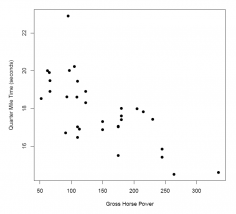
(a) Create a scatter plot of the two variables. What does the pattern of points suggest about the relationship (if any) between the variables? Are there any outliers?

Answer:The scatter plot makes clear that the relationship between gross horse power and quarter-mile time (seconds) is both negative and (approximately) linear. There appears to be one conspicuous outlier in the upper left-hand corner of the plot.

plot(mtcars$hp, mtcars$qsec, pch = 19,
xlab = "Gross Horse Power",
ylab = "Quarter Mile Time (seconds)")

(b) Letting the quarter-mile time be the dependent variable, estimate the regression equation. Write out the regression equation, ŷ = b₀ + b₁x.

reg_eq_mtcars <- lm(qsec ~ hp, data = mtcars)
reg_eq_mtcars
##
## Call:
## lm(formula = qsec ~ hp, data = mtcars)
##
## Coefficients:
## (Intercept) hp
## 20.55635 -0.01846

Answer: The estimated regression equation is: ŷ = 20.5564 – 0.0185x.

summary(reg_eq_mtcars)
##
## Call:
## lm(formula = qsec ~ hp, data = mtcars)
##
## Residuals:
## Min 1Q Median 3Q Max
## -2.1766 -0.6975 0.0348 0.6520 4.0972
##
## Coefficients:
## Estimate Std. Error t value Pr(>|t|)
## (Intercept) 20.556354 0.542424 37.897 < 2e-16 ***
## hp -0.018458 0.003359 -5.495 5.77e-06 ***
## ---
## Signif. codes: 0 ' *** ' 0.001'**' 0.01'*' 0.05'.' 0.1' ' 1
##
## Residual standard error: 1.282 on 30 degrees of freedom
## Multiple R-squared: 0.5016,Adjusted R-squared: 0.485
## F-statistic: 30.19 on 1 and 30 DF, p-value: 5.766e-06

Answer: The r² is 0.502, indicating that approximately 50.2% of variation in the dependent variable is explained by variation in the independent variable.

(d) What is the p-value?

Answer: p-value = 0.00000577

(e) Is the estimated regression equation significant at the α = 0.05 level?

Answer: Since p-value = 0.00000577 is far less than the usual values for (including α = 0.05), we would say that the estimated regression equation is significant.

4. Use the mtcars data set to answer the following questions.

(a) Find the predicted quarter-mile time for all the values of gross horsepower from the data set used in the original analysis. Report the predicted values for the last four observations.

Answer:

tail(fitted(reg_eq_mtcars) , 4)
## Ford Pantera L Ferrari Dino Maserati Bora Volvo 142E
## 15.68336 17.32615 14.37282 18.5444

(b) Find the predicted values of quarter-mile time for the following values of gross horsepower: 100, 125, 160, 225, and 250.

Answer:

new_values <- data.frame(hp <- c(100, 125, 160, 225, 250))
predict(reg_eq_mtcars, new_values)
## 1 2 3 4 5
## 18.71052 18.24906 17.60302 16.40323 15.94178

(c) Can we use the estimated regression equation to make predictions of quartermile time when gross horsepower is 40 or 350? Why or why not?

Answer: When we learn that the minimum and maximum values of the variable hp are 52 and 335, respectively, we should not use the estimated regression equation to make predictions based on values that fall above or below that range. Some analysts will do so anyway, but one should proceed very carefully when making any predictive claims based on this estimated regression equation.

min(mtcars$hp)
## [1] 52
max(mtcars$hp)
## [1] 335

5. This exercise explores the relationship (if any) between two of the five variables comprising the data set polling: x₁ =age, measured in years, and x₃ =same sex, which is measured on a 1-to-7 Likert scale as a response to the statement, "I approve of the right of same-sex couples to marry." A respondent registers strong disapproval with a 1, strong approval with a 7, and relative indi erence with a response in the middle of the range from 1 to 7. (Note: polling can be found on the book's website.)

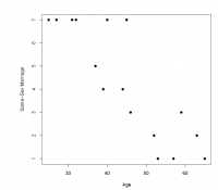
(a) Make a scatter plot of x₃ against x₁. Do you see any possible violations of the assumptions underlying the correct application of simple linear regression analysis? What does the nature of the pattern tell you? Do you think regression can be used to explore the relationship between the two variables?

Answer: The scatter plot reveals the negative and (relatively) linear relationship between a person's age and the extent to which he or she approves of the right of same-sex couples to marry. That is, in general, resistance to the idea that same-sex couples should have the right to marry seems to increase with one's age. However, as with most plots, the relationship is not a perfect one. In particular, we note that the residuals do not appear to be constant for all values of the independent variable. Even so, regression analysis would seem to be a promising means by which to explore the relationship between these two variables.

plot(polling$x1, polling$x3, xlab = "Age", ylab = "Views of
Same-Sex Marriage", pch = 19)

(b) Write out the regression equation. In this case, does it make more sense to specify x₁ or x₃ as the dependent variable? That is, should you de ne the model as x₃ = b₀ + b₁x₁ or as x₁ = b₀ + b₁x₃? Why?

Answer: We would most likely specify x₃, Same-Sex Marriage, as the dependent variable and x₁, Age, as the independent variable. Although we do not use regression analysis to demonstrate causality, it makes more sense to say that approval of the right of same-sex couples to marry falls with age than the reverse.

The estimated regression equation is ŷ = 11.757 – 0.168.

reg_eq_polling <- lm(x3 ~ x1, data = polling)
reg_eq_polling
##
## Call:
## lm(formula = x3 ~ x1, data = polling)
##
## Coefficients:
## (Intercept) x1
## 11.757 -0.168

summary(reg_eq_polling)
##
## Call:
## lm(formula = x3 ~ x1, data = polling)
##
## Residuals:
## Min 1Q Median 3Q Max
## -1.8535 -1.0235 -0.2935 0.6705 2.8025
##
## Coefficients:
## Estimate Std. Error t value Pr(>|t|)
## (Intercept) 11.7573 1.2276 9.577 1.59e-07 ***
## x1 -0.1680 0.0265 -6.340 1.83e-05 ***
## ---
## Signif. codes: 0'***' 0.001'**' 0.01'*' 0.05'.' 0.1 ' '1
##
## Residual standard error: 1.296 on 14 degrees of freedom
## Multiple R-squared: 0.7417,Adjusted R-squared: 0.7232
## F-statistic: 40.19 on 1 and 14 DF, p-value: 1.829e-05

Answer: r² = 0.742

(d) What is the p-value?

Answer: p-value = 0.00001829

(e) Is the regression equation significant at the α = 0.05 level?

Answer: Since p-value = 0.00001829 is less than α = 0.05, we would say that the estimated regression equation is significant.

(f) Find the 95% confidence interval estimate of β₁.

confint(reg_eq_polling, level = 0.95)
## 2.5 % 97.5 %
## (Intercept) 9.1242484 14.3903218
## x1 -0.2248278 -0.1111626

Answer: [ –0.2248, –0.1112]

(g) State in words the meaning of the confidence interval estimate of β₁.

Answer: We can be 95% confident that β₁ falls in the interval from -0.2248 to -0.1112.

(h) What are your conclusions about the regression analysis? Please write out your conclusions in a similar way to those written out in point 6, part (c), of the Summary section above.

Answer: The estimated regression equation ŷ = 11.757 – 0.168x allows us to conclude that a change of 1 year is associated with a change of -0.168 in approval. (We know this because the regression coefficient is b₁ = –0.168.) In this case, the meaning of the intercept term, b₀ = 11.757, is less clear because it represents the predicted value of approval for a person whose age is 0. Even so, it is important to retain the intercept term in the equation because it must be included when we want to make predictions.

Statistics with R

Student Resources

Chapter 12: Simple Linear Regression