Chapter 13: Multiple Regression
1. Consider the estimated regression equation:ŷ = 3536 + 1183x1 – 1208x2. Suppose the model is changed to reflect the deletion of x2 and the resulting estimated simple linear equation becomes ŷ= –10663 + 1386x1.
(a) How should we interpret the meaning of the coefficient on x1 in the estimated simple linear regression equation ŷ= –10663 + 1386x1?
Answer: A one-unit change in the independent variable x1 is associated with an expected change of 1386 units in the dependent variable ŷ.
(b) How should we interpret the meaning of the coecient on x1 in the estimated multiple regression equation ŷ= 3536 + 1183x1– 1208x2?
Answer: A one-unit change in the independent variable x1 is associated with an expected change of 1183 in the dependent variable ŷ if the other independent variable x2 is held constant.
(c) Is there any evidence of multicollinearity? What might that evidence be?
Answer: There is some multicollinearity between x1 and x2 because the co- effcient has changed from 1386 to 1183 with the introduction of x2 into the regression model. In the case when the independent variables are perfectly uncorrelated, the coefficient is unchanged.
2.Interpret the results below and answer the following questions. Suppose we regress the dependent variable y on four independent variables x1, x2, x3, and x4. After running the regression on n = 16 observations, we have the following information: SSreg = 946.181 and SSres = 49.773. Please answer the following questions.
(a) What is the value of r2?
Answer: 0.95
Since SSy = SSreg + SSres = 946.181 + 49.773 = 995.954, we know that

(b) What is the adjusted r2?
Answer: 0.932

(c) What is the F −statistic?
Answer: 52.277

Answer: p-value = 0.0000004338
= p(F > 52.277, 4, 11) = 0.0000004338
pf(52.277, 4, 11, lower.tail = FALSE)
## [1] 4.338219e-07
(e) Is the overall regression model significant? Test at the α = 0.05 level of significance.
Answer: Yes, since p-value = 0.0000004338 < α = 0.05, we conclude that the estimated regression model is significant.
3. Referring to Question 2, suppose we also have the following information about the partial regression coefficients.

(a) Is b1 significant at α = 0.05? What is its t-value? What is its p-value?
Answer: Since t = –0.2718 and p-value = 0.7908 > α = 0.05, b1 is not significant.

2 * pt(-0.2718, 11)
## [1] 0.7908094
(b) Is b2 significant at α = 0.05? What is its t-value? What is its p-value?
Answer: Since t = −2.5875 and p-value = 0.02525 < α = 0.05, b2 is significant.

(c) Is b3 significant at α = 0.05? What is its t-value? What is its p-value?
Answer: Since t = 3.9340 and p-value = 0.002336 < α = 0.05, b3 is significant.

2 * pt(3.9340, 11, lower.tail = FALSE)
## [1] 0.002335972
(d) Is b4 significant at α = 0.05? What is its t-value? What is its p-value?
Answer: Since t = 1.8232 and p-value = 0.09554 > α= 0.05, b4 is not significant.

2 * pt(1.8232, 11, lower.tail = FALSE)
## [1] 0.09553817
4. Consider the estimated multiple regression equation:
ŷ = –0.59141 + 0.05800x1 + 0.84490x2 + 0.11419x3.
(a) Complete the missing entries in this ANOVA table.

Answer: The answers to part (a) are the bolded numbers in the following table.

pf(21.1331, 3, 6, lower.tail = FALSE)
## [1] 0.001366979
(b) Complete the missing entries in this coeffcients table.

Answer: The answers to part (b) are the bolded numbers in the following table.

#p-value for bo
2 * pt(-0.5737, 6)
## [1] 0.5870154
#p-value for b1
2 * pt(5.362, 6, lower.tail = FALSE)
## [1] 0.001724838
#p-value for b2
2 * pt(3.439, 6, lower.tail = FALSE)
## [1] 0.01381786
#p-value for b3
2 * pt(0.823, 6, lower.tail = FALSE)
## [1] 0.4419823
(c) What is the value of r2?
Answer: 0.914

(d) What is the adjusted r2?
Answer: 0.871

5. This exercise uses the mtcars data set that is installed in R.
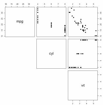
a) Use the pairs() function to create a scatter plot matrix for three variables: mpg, cyl, and wt. What can we say about the relationships between these variables?
We can apply the pairs() function to a subset of mtcars which contains only variables mpg (column 1), cyl (column 2), and wt (column 6). We use the tail() function to identify the column position of each variable.
tail(mtcars, 2)
## mpg cyl disp hp drat wt qsec vs am gear carb
## Maserati Bora 15.0 8 301 335 3.54 3.57 14.6 0 1 5 8
## Volvo 142E 21.4 4 121 109 4.11 2.78 18.6 1 1 4 2
pairs(mtcars[, c(1, 2, 6)], pch = 19, lower.panel = NULL)

Answer: From the scatter plot, it is clear that mpg is negatively related to cyl and wt and that cyl is positively related to wt.
(b) Regress the dependent variable mpg on the variables cyl and wt. Write out the estimated regression equation.
reg_eq_mileage <- lm(mpg ~ cyl + wt, data = mtcars)
reg_eq_mileage
##
## Call:
## lm(formula = mpg ~ cyl + wt, data = mtcars)
##
## Coefficients:
## (Intercept) cyl wt
## 39.686 -1.508 -3.191
Answer: The estimated regression equation is ŷ = 39.69 – 1.51 x1 – 3.19x2, where ŷ is the predicted value of mpg, x1 is cyl, and x2 is wt. That the partial regression coeffcients have a negative sign is unsurprising in view of the scatter plots above.
(c) Use the fitted() function to create the predicted dependent variables for the values of cyl and wt in the original data set. Just to check that the predictions are correct, select two observations and work out the predicted values manually.
predicted <- fitted(reg_eq_mileage)
tail(predicted, 2)
## MaseratiBora Volvo142E
## 16.23213 24.78418
Answer: From part (a), we see that for the Maserati Bora, cyl = 8 and wt = 3.57. Plugging these values into the estimated regression equation, we nd that ŷ= 39.69–1.51x1–3.19x2 = 39.69–1.51(8)–3.19(3.57) = 16.23. For the Volvo 142E, cyl = 4 and wt = 2.78, ŷ = 39.69–1.51(4)–3.19(2.78) = 24.78. Thus, the predicted values of the dependent variable found using the fitted() function exactly equal those found when substituting the values of the independent variables into the estimated regression equation.
(d) Use the predict() function to create the predicted dependent variable for the following pairs of values of the independent variables: for the rst pair cyl = 4 and wt = 5; for the second pair cyl = 8 and wt = 2.
newvalues <- data.frame(cyl = c(4, 8), wt = c(5, 2))
predict(reg_eq_mileage, newvalues)
## 1 2
## 17.70022 21.24196
Answer: To check these predicted values, we simply plug (a) cyl = 4 and wt = 5 and (b) cyl = 8 and wt = 2 into ŷ = 39.69 – 1.51x1 – 3.19x2 and find ŷ in each case: ŷ = 39.69 – 1.51(4) – 3.19(5) = 17.70 and ŷ = 39.69 – 1.51(8) – 3.19(2) = 21.24.


