Chapter 3: Descriptive Statistics: Numerical Methods

1. Use R to find the 90th percentile, the 1st, 2nd, and 3rd quartiles as well as the minimum and maximum values of the LakeHuron data set. (Recall that R has a number of data sets included in its basic installation; LakeHuron is the name of the data set that contains the “level of Lake Huron 1875 - 1972.” To see all the available data sets included in R, simply enter data() at the R prompt in the Console.) What are the mean and median?

Answer:

quantile(LakeHuron, prob = c(0.00, 0.25, 0.50, 0.75, 0.90, 1.00))

##      0%           25%        50%    75%         90%      100%

##  575.960  578.135  579.120  579.875   580.646   581.860

mean(LakeHuron)

##   [1]   579.0041

median(LakeHuron)

##  [1]   579.12

2. Use R to find the range, the interquartile range, the variance, the standard deviation, and the coefficient of variation of the LakeHuron data set.

Answer:

#Comment. Set the number of decimal places (digits) to be reported

options(digits = 4)

max(LakeHuron) - min(LakeHuron)
##  [1]  5.9

IQR(LakeHuron)
##   [1]   1.74

var(LakeHuron)
##  [1]   1.738

sd(LakeHuron)
##   [1]   1.318

sd(LakeHuron) / mean(LakeHuron)
##   [1]   0.002277 

3. Use R to create a vector with the following elements: -37.7, -0.3, 0.00, 0.91, e, π, 5.1, 2e, and 113,754, where e is the base of the natural logarithm (roughly 2.718282...) and π the ratio of a circle’s diameter to its radius (about 3.141593...). Name it E3_2 and find the mean, median, 78th percentile, variance, and standard deviation. Note: R understands exp(1) as e, pi as π.

Answer:

#Comment. Override default of reporting very large (and very small)

#numbers with scientific notation

options(scipen=99)

E3_2 <- c(-37.7, -0.3, 0.00, 0.91, exp(1), pi, 5.1, 2*exp(1), 113754)

mean(E3_2)

##  [1]  12637

median(E3_2)

##  [1]  2.718

quantile(E3_2, prob = c(0.78))

##      78%

##      5.181

var(E3_2)

##  [1]  1437840293

sd(E3_2)

##  [1]   37919

The mean is 12,637; the median is 2.7 or e. Since the data values in E3_2 are arranged in ascending order, the median is easily identified as the middle value, e (or 2.718282...), since there are four values below and four values above. Moreover, simply summing all nine data values, and dividing by nine, provides the mean. The 78th percentile is reported as 5.181; the variance and standard deviation are 1,437,840,293 and 37,919, respectively.

4. Use R to define 2 vectors, x and y, where x contains 24, 22, 22, 21, and 19, and y contains 27, 24, 23, 21, and 19. Which is the most likely correlation coefficient describing the relationship between x and y? -0.90, -0.50, -0.10, 0.00, +0.10, +0.50, or +0.90? Use R to find the correlation and covariance x and y.

Answer:

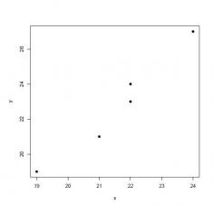
+0.90 is the closest value that the correlation coefficient might assume: the relationship between the two variables is not only positive, it is linear as well. The actual correlation coefficient and plot confirm this relationship.

#Comment1. create vector x 

x <- c(24, 22, 22, 21, 19)

#Comment2. create vector y 

y <- c(27, 24, 23, 21, 19)

#Comment3. using vectors x and y, create data frame data

 data <- data.frame(X = x, Y = y)

#Comment4. examine contents of data frame 

data

##        X    Y

##  1   24   27

##  2   22   24

##  3   22   23

##  4   21   21

##  5   19   19

#Comment5. find correlation coefficient of x and y

cor(data$X, data$Y)

##   [1]   0.98

#Comment6. create the scatter plot of x against y

plot(data$X, data$Y, pch = 19, xlab = 'x', ylab = 'y')

capture.jpg

5. Use R to define a vector with the following elements: 10, 20, 30, 40, 50, 60, 70, 80, 90, 100. Making use of the vectorization capability of R, find the sample variance and sample standard deviation of this set of data. Just to make certain that your answers are correct, check both against those using the functions var() and sd().

#Comment1. define data object E3_3
E3_3 <- seq(from = 10, to = 100, by = 10)

#Comment2. find the variance

xbar <- mean(E3_3)
devs <- (E3_3 - xbar)

sqrd.devs <- (devs)^2
sum.sqrd.devs <- sum(sqrd.devs)
variance <- sum.sqrd.devs / (length(E3_3) - 1)
variance
##   [1]   916.7

#Comment3. find the standard deviation
standard.deviation <- sqrt(variance)
standard.deviation
##   [1]   30.28

#Comment4. find the variance of E3_3 using var() function
var(E3_3)
##   [1]   916.7
#Comment5. find the standard deviation of E3_3 using sd() function sd(E3_3)
##  [1]  30.28

Answer: the variance is 916.7, the standard deviation 30.28.