Chapter 8: Confidence Interval Estimation
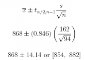
1. According to a survey, the average British household is expected to spend £868 on holiday-related expenses during the Christmas period 2013. This amount covers not only gifts, but also food, beverages, and decorations. Assume the study was based on n = 94 randomly sampled households throughout Great Britain. Assume that the sample standard deviation was £162.
(a) What is the 60% confidence interval estimate of the population mean amount- to-be-spent µ during the Christmas holiday period?
Answer: £868 ± £14.14

(b) What is the 80% confidence interval estimate of the population mean amount-to-be-spent during the same period?
Answer: £868 ± £21.57

(c) What is the 90% confidence interval estimate of the population mean amount- to-be-spent µ during the same period?
Answer: £868 ± £27.75

2. The manager of an insurance office wishes to gain a better understanding of the dollar value of the newly purchased automobiles his firm has insured over the previous 12 months. To this end, he randomly selects 70 insurance applications from the previous year which specified the total cost of each vehicle insured, including market value, taxes, and licensing fees. Use R and the data set insurance from the website to answer the following questions.
(a) Find the 90% confidence interval estimate of the mean dollar value of newly purchased automobiles µ.
Answer: [$17, 027, $20, 221]
t.test(insurance$automobile, conf = 0.90)
##
## One Sample t-test
##
## data: insurance$automobile
## t = 19.443, df = 69, p-value < 2.2e-16
## alternative hypothesis: true mean is not equal to 0
## 90 percent confidence interval:
## 17027.03 20220.97
## sample estimates:
## mean of x
## 18624
(b) Find the 95% confidence interval estimate of the mean dollar value of newly purchased automobiles µ.
Answer: [$16, 713, $20, 535]
t.test(insurance$automobile, conf = 0.95)
##
## One Sample t-test
##
## data: insurance$automobile
## t = 19.443, df = 69, p-value < 2.2e-16
## alternative hypothesis: true mean is not equal to 0
## 95 percent confidence interval:
## 16713.13 20534.87
## sample estimates:
## mean of x
## 18624
(c) Find the 99% confidence interval estimate of the mean dollar value of newly purchased automobiles µ
Answer: [$16, 087, $21, 161]
t.test(insurance$automobile, conf = 0.99)
##
## One Sample t-test
##
## data: insurance$automobile
## t = 19.443, df = 69, p-value < 2.2e-16
## alternative hypothesis: true mean is not equal to 0
## 99 percent confidence interval:
## 16086.66 21161.34
## sample estimates:
## mean of x
## 18624
3. The commute-to-work time for the residents of the world’s large cities has been investigated extensively. A pilot study involving an SRS of residents of Toronto is used to provide an estimate of 10 minutes for the population standard deviation σ. Answer the following questions.
(a) If we want to estimate the population mean commute-to-work time µ for the residents of Toronto with a margin of error of 2 minutes, what sample size n should you recommend? Assume 90% confidence.
Answer: n = 68

Check:

(b) If we want to estimate the population mean commute-to-work time µ for the residents of Toronto with a margin of error of 1 minute, what sample size n should you recommend? Assume 90% confidence.
Answer: n = 271

Check:

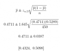
4. In a study of consumer confidence among middle-class Indian families, 450 were interviewed in the metropolitan area of Mumbai. When asked about having to cut back on discretionary purchases of big-ticket items, 212 of 450 responded that their families had done so over the previous 6 months.
(a) What is the 90% confidence interval estimate of the population proportion p of this type of household cutting back on discretionary spending?
Answer: 0.4711 ± 0.0387


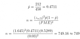
(b) What sample size would you recommend to achieve a margin of error of 0.03?
Answer: n = 749

Check:

(c) How large a sample size would be required to achieve a 99% confidence interval estimate of p with a margin of error of 0.03?
Answer: n = 1, 836

Check:

(d) How large a sample size would be required to achieve a 99% confidence interval estimate of p with a margin of error of 0.025?
Answer: n = 2, 643


Check:

5. A human resources manager at a small university in the US has been considering a change to the structure of employee benefits (in terms of healthcare coverage and pension savings). To get an idea of how receptive the faculty, administrators, and staff members might be to the proposed changes, she has decided to conduct a survey in which n = 188 respondents could register their support or opposition. Use R and the data set benefits from the website to answer the following questions.
(a) Find the 90% confidence interval of p.
Answer: [0.5692, 0.6861]
t.test(benefits$agree, conf.level = 0.90)
##
## One Sample t-test
##
## data: benefits$agree
## t = 17.755, df = 187, p-value < 2.2e-16
## alternative hypothesis: true mean is not equal to 0
## 90 percent confidence interval:
## 0.5692216 0.6860976
## sample estimates:
## mean of x
## 0.6276596
(b) Find the 95% confidence interval of p.
Answer:[0.5579, 0.6974]
t.test(benefits$agree, conf.level = 0.95)
##
## One Sample t-test
##
## data: benefits$agree
## t = 17.755, df = 187, p-value < 2.2e-16
## alternative hypothesis: true mean is not equal to 0
## 95 percent confidence interval:
## 0.5579200 0.6973991
## sample estimates:
## mean of x
## 0.6276596
(c) Find the 99% confidence interval of p.
Answer: [0.5357, 0.7197]
t.test(benefits$agree, conf.level = 0.99)
##
## One Sample t-test
##
## data: benefits$agree
## t = 17.755, df = 187, p-value < 2.2e-16
## alternative hypothesis: true mean is not equal to 0
## 99 percent confidence interval:
## 0.5356609 0.7196582
## sample estimates:
## mean of x
## 0.6276596

