Statistics with R
Student Resources
Chapter 3: Descriptive Statistics: Numerical Methods
1. A sample contains the following data values: 1.50, 1.50, 10.50, 3.40, 10.50, 11.50, and 2.00. What is the mean? Create an object named E3_1; apply the mean() function.
#Comment1. Use the c() function; read data values into object E3_1.
E3_1 <- c(1.50, 1.50, 10.50, 3.40, 10.50, 11.50, 2.00)
#Comment2. Use the mean() function to find the mean.
mean(E3_1)
## [1] 5.842857
Answer: The mean is 5.843.
2. Find the median of the sample (above) in two ways: (a) use the median() function to find it directly, and (b) use the sort() function to locate the middle value visually.
#Comment1. Use the median() function to find the median.
median(E3_1)
## [1] 3.4
#Comment2. Use the sort() function to arrange data values in
#ascending order.
sort(E3_1)
## [1] 1.5 1.5 2.0 3.4 10.5 10.5 11.5
Answer: The median of a data set is the middle value when the data items are arranged in ascending order. Once the data values have been sorted into ascending order (we have done this above using the sort() function) it is clear that the middle value is 3.4 since there are 3 values to the left of 3.4 and 3 values to the right. Alternatively, the function median() can be used to find the median directly.
3. Create a vector with the following elements: -37.7, -0.3, 0.00, 0.91, e, π, 5.1, 2e and 113,754, where e is the base of the natural logarithm (roughly 2.718282...) and the ratio of a circle's diameter to its radius (about 3.141593...). Name the object E3_ 2. What are the median and the mean? The 78th percentile? What are the variance and the standard deviation? Note that R understands exp(1) as e, pi as π.
#Comment1. Use the c() function to create the object E3_2.
E3_2 <- c(-37.7, -0.3, 0.00, 0.91, exp(1), pi, 5.1, 2*exp(1), 113754)
#Comment2. Use the mean() function to find the mean.
mean(E3_2)
## [1] 12637.03
#Comment3. Use the median() function to find the median.
median(E3_2)
## [1] 2.718282
#Comment4. Use the quantile() function with prob = c(0.78)
#to find the 78th percentile.
quantile(E3_2, prob = c(0.78))
## 78%
## 5.180775
#Comment5. Use the var() function to find the variance.
var(E3_2)
## [1] 1437840293
#Comment6. Use the sd() function to find the standard deviation.
sd(E3_2)
## [1] 37918.86
Answer: The mean is 12,637.03; the median is 2.718282..., or e. Since the data values in E3_ 2 are arranged in ascending order, the median is easily identifed as the middle value, e (or 2.718282...), since there are four values below and four values above. Moreover, simply summing all nine data values, and dividing by nine, provides the mean. The 78th percentile is reported as 5.180775; the variance and standard deviation are 1,437,840,293 and 37,918.86, respectively.
4. Consider the following data values: 10, 20, 30, 40, 50, 60, 70, 80, 90, and 100. What are the 10th and 90th percentiles? Hint: use function seq(from=,to=,by=) to create the data set. Name the data set E3_3.
#Comment1. Use the seq(from =, to =, by =) function to create
#object E3_3
E3_3 <- seq(from = 10, to = 100, by = 10)
#Comment2. Examine the contents of E3_3 to make sure it contains
#the desired elements.
E3_3
## [1] 10 20 30 40 50 60 70 80 90 100
#Comment3. Use the quantile() function to find the 10th and 90th
#percentiles. Remember to use probs=c(0.1, 0.9)
quantile(E3_3, probs = c(0.1, 0.9))
## 10% 90%
## 19 91
Answer: The 10th and 90th percentiles are 19 and 91, respectively. Note that the 10th percentile (19) is a value which exceeds at least 10% of items in the data set; the 90th percentile (91) is a value which exceeds at least 90% of the items. Note also that it is possible to define any percentiles by setting the values in the probs=c() argument of the quantiles() function.
5. What is the median of E3_3? Find the middle value visually and with the median() function.
#Comment. Use function median() to find the median.
median(E3_3)
## [1] 55
Answer: This data set has an even number of values, all arranged in ascending order. Accordingly, the median is found by taking the average of the values in the two middle positions: the average of 50 (the value in the 5th position) and 60 (the value in the 6th position) is 55.
6. The mode is the value that occurs with greatest frequency in a set of data, and it is used as one of the measures of central tendency. Consider a sample with these nine values: 5, 1, 3, 9, 7, 1, 6, 11, and 8. Does the mode provide a measure of central tendency similar to that of the mean? The median?
#Comment1. Use the c() function and read the data into object E3_4.
E3_4 <- c(5, 1, 3, 9, 7, 1, 6, 11, 8)
#Comment2. Use the table() function to create a frequency
#distribution.
table(E3_4)
## E3_4
## 1 3 5 6 7 8 9 11
## 2 1 1 1 1 1 1 1
#Comment3. Use the mean() and median() functions to find the
#mean and median of E3_4.
mean(E3_4)
## [1] 5.666667
median(E3_4)
## [1] 6
Answer: Since the value of the mode in this instance is 1 (it appears twice), it provides less insight into the central tendency of this sample than does the mean (5.667) or the median (6).
7. Consider another sample with these nine values: 5, 1, 3, 9, 7, 4, 6, 11, and 8. How well does the mode capture the central tendency of this sample?
Answer: Since all the data items appear only once, there is no single value for the mode; there are nine modes, one for each data value.
8. Find the 90th percentile, the 1st, 2nd, and 3rd quartiles as well as the minimum and maximum values of the LakeHuron data set (which is part of the R package and was used in the Chapter 1 in-text exercises). What is the mean? What is the median?
#Comment1. Use the quantile() function with prob=c().
quantile(LakeHuron, prob = c(0.00, 0.25, 0.50, 0.75, 0.90, 1.00))
## 0% 25% 50% 75% 90% 100%
## 575.960 578.135 579.120 579.875 580.646 581.860
#Comment2. Use the mean() function to find the mean.
mean(LakeHuron)
## [1] 579.0041
#Comment3. Use the median() function to find the median.
median(LakeHuron)
## [1] 579.12
Answer: The minimum value (the 0 percentile) is 575.960 and the maximum value (the 100th percentile) is 581.860; the 1st, 2nd, and 3rd quartiles are 578.135, 579.120, and 579.875, respectively. The median (also known as the 2nd quartile or the 50th percentile) is 579.120. The mean is 579.0041 while the 90th percentile is 580.646.
9. Find the range, the interquartile range, the variance, the standard deviation, and the coefficient of variation of the LakeHuron data set.
#Comment1. Find the range by subtracting min() from max().
max(LakeHuron) - min(LakeHuron)
## [1] 5.9
#Comment2. Use the IQR() function to find the interquartile range.
IQR(LakeHuron)
## [1] 1.74
#Comment3. Use the var() function to find the variance.
var(LakeHuron)
## [1] 1.737911
#Comment4. Use the sd() function to find the standard deviation.
sd(LakeHuron)
## [1] 1.318299
#Comment5. To find the coefficient of variation, find sd()/mean().
sd(LakeHuron) / mean(LakeHuron)
## [1] 0.002276838
Answer: The range is 5.9 feet and the interquartile range is 1.74 feet. Moreover, the variance and standard deviation are 1.737911 and 1.318299 feet, respectively. Finally, the coeffcient of variation is 0.002276838; that is, the standard deviation is only about 0.228% of the mean.
10. What are the range and interquartile range for the following data set: -37.7, -0.3, 0.00, 0.91, e, π, 5.1, 2e and 113,754? Note that this is the same data set as that used above where we named it E3_2.
#Comment1. To find range, subtract min() from max().
max(E3_2) - min(E3_2)
## [1] 113791.7
#Comment 2. To find interquartile range, use IQR() function.
IQR(E3_2)
## [1] 5.1
Answer: The range is 113,791.7; the interquartile range is 5.1. The great difference between these two measures of dispersion results from the fact that the interquartile range provides the range of the middle 50% of the data while the range includes all data values, including the outliers.
11.Using the vectorization capability of R, find the sample variance and sample standard deviation of the data set E3_3 (used above). (This exercise provides the opportunity to write and execute some basic R code for the purpose of deriving the variance and standard deviation of a simple data set.) Check both answers against those using the var() and sd() functions. Recall that the expression for the sample
variance is

#Comment1. Use mean() to find mean of E3_3; assign to xbar.
xbar <- mean(E3_3)
#Comment2. Find the deviations about the mean; assign to devs.
devs <- (E3_3 - xbar)
#Comment3. Find the squared deviations about the mean; assign
#the result to sqrd.devs.
sqrd.devs <- (devs) ^ 2
#Comment4. Sum the squared deviations about the mean; assign
#result to the object sum.sqrd.devs.
sum.sqrd.devs <- sum(sqrd.devs)
#Comment5. Divide the sum of squared deviations by (n-1)
#to find the variance; assign result to the object variance.
variance <- sum.sqrd.devs / (length(E3_3) - 1)
#Comment6. Examine the contents of variance.
variance
## [1] 916.6667
#Comment7. The standard deviation is the positive square root
#of the variance; assign result to the object standard.deviation.
standard.deviation <- sqrt(variance)
#Comment8. Examine the contents of standard.deviation.
standard.deviation
## [1] 30.2765
#Comment9. Use the var() function to find the variance.
var(E3_3)
## [1] 916.6667
#Comment10. Use the sd() function to find the standard
#deviation.
sd(E3_3)
## [1] 30.2765
Answer: The variance is 916.6667; the standard deviation is 30.2765. The answers reported by var() and sd() equal those produced by way of vectorization.
12. The temps data set (available on the companion website) includes the high-and-low temperatures (in degrees Celsius) for April 1, 2016 of ten major European cities; import the data set into an object named E3_5. What is the covariance of the high and low temperatures? What does the covariance tell us?
Answer: The covariance of the two variables is 37.28889. Although it is difficult to learn very much from the value of the covariance of the two variables, we do know that the two variables are positively related. This is an unsurprising nding because the cities having the warmest daytime temperatures are also those that have the warmest nighttime temperatures.
#Comment1. Read data set temps into the object named E3_5.
E3_5 <- temps
#Comment2. Use the head(,3) function to find out the variable names.
head(E3_5, 3)
## City Daytemp Nighttemp
## 1 Athens 21 12
## 2 Barcelona 12 9
## 3 Dublin 6 1
#Comment3. Use the cov() function to find the covariance. The
#variable names are Daytemp and Nighttemp.
cov(E3_5$Daytemp, E3_5$Nighttemp)
## [1] 37.28889
13. To gain practice using R, calculate the covariance of the two variables in the temps data (available on the companion website). Do not use the function cov(). Recall that the sample covariance between two variables x and y is:

Answer:
#Comment1. Find the deviations between each observation
#on Daytemp and its mean. Name resulting object devx.
devx <- (E3_5$Daytemp - mean(E3_5$Daytemp))
#Comment2. Find the deviations between each observation
#on Nighttemp and its mean. Name resulting object devy.
devy <- (E3_5$Nighttemp - mean(E3_5$Nighttemp))
#Comment3. Find product of devx and devy; name result crossproduct.
crossproduct <- devx * devy
#Comment4. Find the covariance by dividing crossproduct by (n-1),
# or 9. Assign the result to object named covariance.
covariance <- sum(crossproduct) / (length(E3_5$Daytemp) - 1)
#Comment5. Examine contents of covariance. Confirm that it is
#the same value as that found in previous exercise.
covariance
## [1] 37.28889
14. There are several ways we might explore the relationship between two variables. In the next few exercises, we analyze the daily_ idx_ chg data set (available on the companion website) to explore the pros and cons of several of those methods. The data set itself consists of the percent daily change (from the previous trading day) of the closing numbers for two different widely-traded stock indices, the Dow Jones Industrial Average and the S&P500, for all trading days from April 2 to April 30, 2012. Comment on the data. What is the covariance of the price movements for the two indices? What does the covariance tell us about the relationship between the two variables? As a first step, import the data into an object named E3_6.
#Comment1. Read the daily_idx_chg data into the object E3_6.
E3_6 <- daily_idx_chg
#Comment2. Use the summary() function to identify the variable names
#and to acquire a feel for what the data look like.
summary(E3_6)
## PCT.DOW.CHG PCT.SP.CHG
## Min. :-1.6500 Min. :-1.7100
## 1st Qu.:-0.6675 1st Qu.:-0.6525
## Median : 0.0350 Median :-0.0550
## Mean : 0.0045 Mean :-0.0340
## 3rd Qu.: 0.6075 3rd Qu.: 0.6875
## Max. : 1.5000 Max. : 1.5500
#Comment3. Use the cov() function to find the covariance.
cov(E3_6)
## PCT.DOW.CHG PCT.SP.CHG
## PCT.DOW.CHG 0.7542682 0.7693505
## PCT.SP.CHG 0.7693505 0.8562042
Answer: The two variable names are PCT.DOW.CHG and PCT.SP.CHG; the data values seem to be centered around 0 with values ranging from around 1.55 to -1.71 The covariance is 0.7693505 which tells us only that the two variables are positively related.
15. Standardize the daily_idx_chg data and re-calculate the covariance. Is it the same?
#Comment1. Use the scale() function to standardize the data.
#Assign the result to the object named std_indices.
std_indices <- scale(E3_6)
#Comment2. Use the cov() function to find the covariance.
cov(std_indices)
## PCT.DOW.CHG PCT.SP.CHG
## PCT.DOW.CHG 1.0000000 0.9573543
## PCT.SP.CHG 0.9573543 1.0000000
Answer: The covariance is 0.9573543. No, the covariance is not the same, even though it has been applied to the same data. In fact, the covariance on raw data does not (in general) equal the covariance on the same data when standardized.
16. Find the correlation of the two variables in the daily _idx_ chg data.
#Comment. Use the cor() function to find the correlation.
cor(E3_6)
## PCT.DOW.CHG PCT.SP.CHG
## PCT.DOW.CHG 1.0000000 0.9573543
## PCT.SP.CHG 0.9573543 1.0000000
Answer: The correlation is 0.9573543, exactly the same as the covariance of the standardized variables. In general, the correlation of two unstandardized variables equals the covariance of the same two variables in standardized form.
17. Standardize the daily _idx_ chg data and re-calculate the correlation. Is it the same?
#Comment. Use the cor() function to find the correlation.
cor(std_indices)
## PCT.DOW.CHG PCT.SP.CHG
## PCT.DOW.CHG 1.0000000 0.9573543
## PCT.SP.CHG 0.9573543 1.0000000
Answer: The correlation between the standardized values is exactly the same as the correlation between the unstandardized values: 0.9573543. While the covariance is a ected by how the data are scaled—making it more dicult to interpret—the correlation is not a affected.
18. Make a scatter plot of the daily idx_ chg_ data with PCT.DOW.CHG on the horizontal axis, PCT.SP.CHG on the vertical. Add a main title and labels for the horizontal and vertical axes. Does the scatter plot con rm the positive linear association suggested by the correlation coeffcient?
#Comment. Use the plot() function to produce the scatter plot.
plot(E3_6$PCT.DOW.CHG, E3_6$PCT.SP.CHG,
xlab ='Percentage Daily Change in the Dow',
ylab ='Percentage Daily Change in the S&P500',
pch = 19,
col ='purple',
main ='A Plot of Daily Percent Changes in the Dow and S&P500')
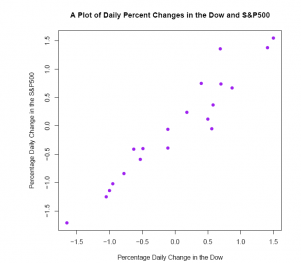
Answer: The scatter plot is consistent with a correlation coefficient of 0.9573543. There is a strongly positive linear association between the two stock market indices.
19. Below we have a curvilinear relationship where the points can be connected with a smooth, parabolic curve. See scatter plot. Which is the most likely correlation coefficient describing this relationship? -0.90, -0.50, -0.10, 0.00, +0.10, +0.50, or +0.90. (In the next four exercises, the code producing the scatter plots is included.)
x <- c(0, -1, -2, -3, -4)
y <- c(4, 2, 1, 2, 4)
data <- data.frame(X = x, Y = y)
plot(data$X, data$Y, pch = 19, xlab ='x', ylab ='y')
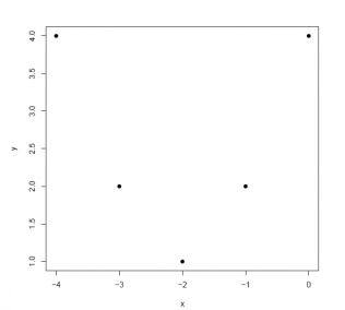
Answer: The correlation coefficient is 0.00.
cor(data$X, data$Y)
## [1] 0
Despite the points being scattered in a way characterized by a curvilinear relationship, the correlation coefficient describes the strength of the linear relationship between two variables. Just because a correlation coecient is zero does not mean that there is no relationship between the two variables. As we see in this case, there may be a relationship that is curvilinear rather than linear.
20. Which is the most likely correlation coefficient describing the relationship below?
See the scatter plot. -0.90, -0.50, -0.10, 0.00, +0.10, +0.50, or +0.90.
x <- c(16, 13, 8, 6, 5)
y <- c(15, 20, 25, 25, 30)
data <- data.frame(X = x, Y = y)
plot(data$X, data$Y, pch = 19, xlab ='x', ylab ='y')
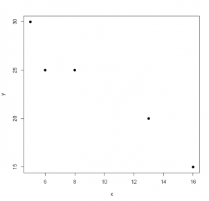
Answer: -0.90 is the closest value that the correlation coefficient might take: the relationship between the two variables is not only negative, it is linear as well. In fact, the correlation coefficient is -0.9657823.
cor(data$X, data$Y)
## [1] -0.9657823
21. Which is the most likely correlation coefficient describing the relationship below?
-0.90, -0.50, -0.10, 0.00, +0.10, +0.50, or +0.90?
x <- c(24, 22, 22, 21, 19)
y <- c(27, 24, 23, 21, 19)
data <- data.frame(X = x, Y = y)
plot(data$X, data$Y, pch = 19, xlab ='x', ylab ='y')
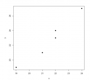
Answer: +0.90 is the closest value that the correlation coefficient might take: the relationship between the two variables is not only positive, it is linear as well.
cor(data$X, data$Y)
## [1] 0.9800379
In fact, the correlation coefficient is +0.9800379.
22. Which is the most likely correlation coefficient describing the relationship below?
-0.90, -0.50, -0.10, 0.00, +0.10, +0.50, or +0.90.
x <- c(0, -30, -30, -30, -60)
y <- c(-20, 10, -20, -50, -20)
data <- data.frame(X = x, Y = y)
plot(data$X, data$Y, pch = 19, xlab ='x', ylab ='y')
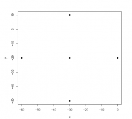
Answer: Although there is a pattern of points in the scatter diagram, there is no discernable linear relationship. In fact, the correlation coefficient is 0.00.
cor(data$X, data$Y)
## [1] 0
23. The Empirical Rule states that approximately 68% of values of a normally-distributed variable fall in the interval from 1 standard deviation below the mean to 1 standard deviation above the mean. (A slightly more precise percentage is 68.269%.) Verify this claim by (a) generating n = 1, 000, 000 normally-distributed values with a mean of 100 and standard deviation of 15, and then (b) "counting" the number of data values that fall in this interval. If this claim is true, then approximately (0.68269)(1, 000, 000) = 682, 690 values should fall in the interval from 85 to 115; roughly (0.15866)(1, 000, 000) = 158, 655 below 85; and approximately (0.15866)(1, 000, 000) = 158, 655 values above 115. Use the rnorm(1000000,100,15) function.
#Comment1. Use the rnorm() function to generate n=1,000,000
#normally-distributed data values with a mean of 100 and standard
#deviation of 15; name the resulting object normal_data.
normal_data <- rnorm(1000000, 100, 15)
#Comment2. Count the number of data values in the object named
#normal_data that are at least 1 standard deviation below the
#mean (that is, at least 15 below 100, or 85). Name this value a.
a <- length(which(normal_data <= 85))
#Comment3. Examine the contents of a to confirm that it is near
#15.866 percent of 1,000,000, or roughly 158,666.
a
## [1] 158607
#Comment4. Count the number of data values in the object named
#normal_data that are at least 1 standard deviation above the
#mean (that is, at least 15 above 100, or 115). Name this value b.
b <- length(which(normal_data >= 115))
#Comment5. Examine the contents of b to confirm that it is near
#15.866 percent of 1,000,000, or roughly 158,666.
b
## [1] 158334
#Comment6. Calculate the proportion of 1,000,000 data items that
#fall in the interval from 1 standard deviation below the mean to
#1 standard deviation above the mean. Name that proportion c.
c <- (1000000 - (a + b)) / 1000000
#Comment7. Examine the contents of c. To ensure that we understand
#how c is calculated, plug the values for a (Comment3) and b
#(Comment5) into the expression for c (Comment6).
c
## [1] 0.683059
Using the data generation capability of R, we can confirm that the proportion of data values falling in the interval from one standard deviation below the mean to one standard deviation above the mean is approximately 68%.
24. The Empirical Rule also tells us that approximately 95% of values of a normally- distributed variable fall in the interval from 2 standard deviations below the mean to 2 standard deviations above the mean. (A more precise percentage is 95.45%.) Verify this claim. If this claim is true, then approximately (0.9545)(1, 000, 000) = 954, 500 values should fall in the interval from 70 to 130; roughly (0,02275)(1, 000, 000) = 22, 750 below 70; and approximately (0.02775)(1, 000, 000) = 22, 750 above 130.
Answer:
#Comment1. Count the number of data values in normal_data that
#are at least 2 standard deviations below the mean (that is, at
#least 30 below 100, or 70); name this object a.
a <- length(which(normal_data <= 70))
#Comment2. Examine the contents of a. Is it near 22,750?
a
## [1] 22762
#Comment3. Count the number of data values in normal_data that
#are at least 2 standard deviations above the mean (that is, at
#least 30 above 100, or 130); name this object b.
b <- length(which(normal_data >= 130))
#Comment4. Examine the contents of b. Is it near 22,750?
b
## [1] 22717
#Comment5. Calculate the proportion of 1,000,000 data items that
#fall in the interval from 2 standard deviations below the mean to
#2 standard deviations above the mean. Name that proportion c.
c <- (1000000 - (a + b)) / 1000000
#Comment6. Examine the contents of c. Is it near 0.9545?
c
## [1] 0.954521
The proportion of data values falling in the interval from two standard deviations below the mean to two standard deviations above the mean is approximately 95:45%.
25. Use the R data generation function to draw n = 1, 000, 000 values from a uniform distribution that runs from a = 75 to b = 125; import the 1,000,000 data values into an object named uniform_data.
To help you envision uniformly-distributed data running between 75 and 125, see the histogram below. Also, see the Chapter 2 Appendix for an example of how the runif() function is used to simulate data values.
#Comment1. Use the runif() function to generate n=1,000,000
#uniformly-distributed data values over the interval from 75 to
#125; name the resulting object uniform_data.
uniform_data <- runif(1000000, 75, 125)
#Comment2. To visualize how the data values are distributed,
#use the hist() function to create a picture of the distribution.
hist(uniform_data,
breaks = 50,
xlim = c(70, 130),
ylim = c(0, 25000),
col ='blue')
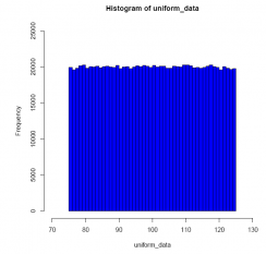
What is the proportion of values that falls in the interval from 90 to 110?
Answer: From this simulation exercise, we see that the proportion of uniformly- distributed data values (running from 75 to 125) that falls in the interval from 90 to 110 is (roughly) 0.40.
#Comment1. Count the number of data values in uniform_data that
#are less than or equal to 90 (that is, all the data values that
#fall in interval from 75 to 90); name this object a.
a <- length(which(uniform_data <= 90))
#Comment2. Examine the contents of a. Is it near 300,000?
a
## [1] 300090
#Comment3. Count the number of data values in uniform_data that
#are greater than or equal to 110 (that is, all the data values
#that fall in the interval from 110 to 125); name this object b.
b <- length(which(uniform_data >= 110))
#Comment4. Examine the contents of b. Is it near 300,000?
b
## [1] 299374
#Comment5. Calculate the proportion of 1,000,000 data values that
#fall in the interval from 90 to 110. Name that proportion c.
c <- (1000000 - (a + b)) / 1000000
#Comment6. Examine the contents of c. Is it near 0.40?
c
## [1] 0.400536
From the histogram, we see that a uniformly-distributed variable assumes the "shape" of a rectangle, and therefore the proportion of data values falling in any interval is directly proportional to the length of that interval. In this case, since the question concerns the proportion of data values in an interval of width 20 (= 110 - 90) for a distribution of width 50 (= 125 - 75), the proportion of data values falling in the
interval from 90 to 110 is 20/50 or 0.40.
