Chapter 2: Descriptive Statistics: Tabular and Graphical Methods

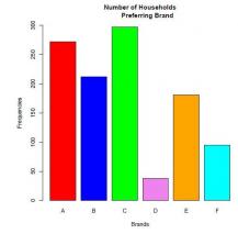
1. A survey of 1,095 households investigating attitudes toward 6 brands,A, B, C, D, E and F,in a certain product category reveals the following preference structure: of the 1,095 households , 272 express a preference for brand A; 212 prefer B; 297 prefer C; 38 prefer D; 181 prefer E; and 95 prefer F. 

a. Use R to create a character vector containing all 1,095 items; name it E2_1.

Answer:

E2_1 <- c(rep('A', 272), rep('B', 212), rep('C', 297), rep('D', 38), rep('E', 181), rep('F', 95))

b.Confirm that E2_1 includes the desired information. Hint: there are many ways this could be done but in this case use the table() function to report the frequency distribution. Since we use it again below, assign the result to the object fd (for frequency distribution) and report the contents of fd.

Answer:

#Comment1. create frequency distribution; store in fd
fd <- table(E2_1)
#Comment2. examine contents of fd
fd
## E2_1
##   A       B      C       D    E     F
##  272   212   297   38  181  95

2. Use fd for all parts of exercise 

a. Produce the relative frequency distribution of E2 _1. Store result in object rf (for relative frequency distribution).

Answer:

#Comment1. set option for the number of decimal places reported
options(digits = 2)
#Comment2. divide fd by sum(fd), the number of elements in fd
#(n=1,049), to find relative frequencies
rf <- fd / sum(fd)
#Comment3. examine contents of rf
rf
## E2_1
##       A         B       C        D        E         F
##  0.248  0.194  0.271  0.035  0.165  0.087

b. Produce a bar graph of frequencies for E2 _1. Color the 6 bars, from left to right: red, blue, green, violet, orange, and cyan. Use argument ylim=c(0, 300) to set scale of vertical axis; use main=‘’ to specify a main title; use xlab=‘’ and ylab=‘’ to define the labels for the horizontal (x), and vertical (y) axes, respectively.

Answer:

barplot(fd, col = c('red','blue', 'green', 'violet', 'orange', 'cyan'), ylim = c(0, 300), main = 'Number of  Households Preferring Brand', xlab = 'Brands', ylab = 'Frequencies')

capture_11.jpg

3. Produce a bar graph of relative frequencies for E2_1. Color the bars brown and purple, alternatively; set vertical axis from 0 to 0.35; include a main title and define labels for the horizontal and vertical axes, respectively. Hint: use rf.

Answer: 

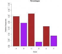
barplot(rf, col = c('brown', 'purple', 'brown', 'purple', 'brown', 'purple'), ylim = c(0, 0.35), main = 'Percentages', xlab = 'Brand', ylab = 'Relative Frequencies')

fig.jpg

4. Use the Cars93 data set (included in the MASS package) to answer the next questions.

a. Use names(Cars93) function to print out the variable names of Cars93.

Answer: 

library("MASS")

##

## Attaching package: ’MASS’

## The following object is masked from ’package:introstats’:

##

##          housing

names(Cars93)

##     [1]   "Manufacturer"            "Model"                        "Type"

##     [4]     "Min.Price"                 "Price"                         "Max.Price"

##     [7]     "MPG.city"                 "MPG.highway"           "AirBags"

##   [10]     "DriveTrain"                "Cylinders"                 "EngineSize"

##   [13]     "Horsepower"              "RPM"                       "Rev.per.mile"

##   [16]     "Man.trans.avail"        "Fuel.tank.capacity"    "Passengers"

##   [19]      "Length"                     "Wheelbase"               "Width"

##  [22]       "Turn.circle"               "Rear.seat.room"         "Luggage.room"

##  [25]       "Weight"                      "Origin"                       "Make"

b. Provide the frequency and relative frequency distributions for the variable Type. What percentage are large cars?

Answer: 

#Comment1. use table() function to create frequency distribution

fd <- table(Cars93$Type)

#Comment2. examine contents of fd (the frequency distribution) fd

##

##         Compact   Large Midsize             Small Sporty               Van

##             16            11             22             21            14               9

#Comment3. create relative frequencies by dividing fd by total

rf <- fd / sum(fd)

#Comment4. examine rf (relative frequency distribution)

rf

##

##         Compact     Large Midsize        Small Sporty     Van

##        0.172            0.118   0.237       0.226   0.151      0.097

The relative frequency distribution shows that 11.8% of vehicles are large.

c. Provide a cross-tabulation table in which the variables Origin and Type are organized along the two margins. Are most of the vehicles of US-origin?

Answer:

table(Cars93$Origin, Cars93$Type)
##
##                     Compact Large Midsize Small Sporty Van
## USA                      7        11            10      7       8       5
## non-USA               9          0           12     14       6     4

As the cross-tabulation table indicates, all of the large vehicles are of US-origin.

5. Using the data set poverty (from https://study.sagepub.com/stinerock), pro- duce a scatter plot with Wind on the horizontal axis and Poverty on the vertical. Label the horizontal and vertical axes as “Wind” and “Percent Below Poverty Line,” respectively. Also, set the color of the points as blue, and express the points as empty circles. (Hint: you can enter ?pch at the prompt in the Console to inspect the various plotting characteristics.)

Answer:

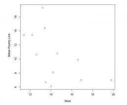
plot(poverty$Wind, poverty$Poverty,xlab = 'Wind', ylab = 'Percent Below Poverty Line', pch = 1, col = 'blue')

fig2.jpg