Chapter 7: Point Estimation and Sampling Distributions
1. Draw a random sample of n = 9 from the tv_hours data set (located on the companion website). Apply function data[sample(nrow(data),n ),]. Assign the values to the object named E7_1.
2. Draw a second random sample of n = 9. Use data[sample(nrow(data),n),]. Assign the values to the object named E7_2.
4. Referring to E7_1, E7_2, and the tv_hours data set, answer the following questions.
(b) What is the sampling error ![]() for both random samples (that is, from both E7_1 and E7_2)?
for both random samples (that is, from both E7_1 and E7_2)?
5. During the 2012 U.S. Presidential Election, 1,500 voters were interviewed upon exiting from a Manhattan polling station where they had just cast their votes. (The data set is named exit and is available on the companion website.) The data are recorded as a 1 for a Barack Obama vote and a 0 for a Mitt Romney vote. Draw a random sample of n = 25. Apply function data[sample(nrow(data),n),]; assign the values to the object named E7_3.
6. Draw a second random sample of n = 25 from exit and assign the values to the object named E7_4. (Remember: be sure to use the data[sample(nrow(data),n),] function.)
9. Suppose a random sample consists of the following 12 elements: 37, 14, 54, 91, 13, 88, 4, 16, 62, 18, 88, and 99. Copy and paste these values into the R Console and store them in an object named E7_5. Once this has been done, add the variable name values and create a data frame named E7_6. Answer the following questions using E7_6. (This exercise is intended to provide a bit of review of material covered earlier.)
Answer: ![]()

#Comment1. Use c() function to create the object E7_5.
E7_5 <- c(37, 14, 54, 91, 13, 88, 4, 16, 62, 18, 88, 99)
#Comment2. Examine contents of E7_5.
E7_5
## [1] 37 14 54 91 13 88 4 16 62 18 88 99
#Comment3. Use data.frame() function to create the data frame
#named E7_6. The variable name is values.
E7_6 <- data.frame(values = E7_5)
#Comment4. Examine the contents of E7_6.
E7_6
## values
## 1 37
## 2 14
## 3 54
## 4 91
## 5 13
## 6 88
## 7 4
## 8 16
## 9 62
## 10 18
## 11 88
## 12 99
#Comment5. What is the point estimate of the population mean?
mean(E7_6$values)
## [1] 48.66667
Answer: s = 35.98

#Comment. Use sd() to calculate the sample standard deviation.
sd(E7_6$values)
## [1] 35.97811
10. When an Iberian tourism authority wanted to know from where travelers on one of their superhighways were coming, they monitored the bridge traffic connecting Castro Marim, Portugal with Ayamonte, Spain (crossing the River Guadiana). They found that for a random sample of 1,062 vehicles, 377 had Portuguese license plates while 418 had Spanish plates. The remaining 267 vehicles had plates from a country other than Spain or Portugal.
Answer: ![]()
![]()
Answer: ![]()
![]()
Answer: ![]()
![]()
11. A random sample of size n = 36 is drawn from a population with a mean of µ = –17 and a standard deviation of σ = 6.
(a) What is ![]()
Answer: 0.8413
![]()
#Comment. Use function pnorm(-16,-17,6/sqrt(36)).
pnorm(-16, -17, 6 / sqrt(36))
## [1] 0.8413447
(b) What is ![]()
Answer: 0.9772
![]()
#Comment. 1 minus pnorm(-19,-17,6/sqrt(36)).
1 - pnorm(-19, -17, 6 / sqrt(36))
## [1] 0.9772499
(c) What is ![]()
Answer: 0.6827
![]()
#Comment. Subtract pnorm(-18,-17,6/sqrt(36)) from
#pnorm(-16,-17,6/sqrt(36))
pnorm(-16, -17, 6 / sqrt(36)) – pnorm(-18, -17, 6 / sqrt(36))
## [1] 0.6826895
(d) What is ![]()
Answer: 0.9545
![]()
#Comment. Subtract pnorm(-19,-17,6/sqrt(36)) from
#pnorm(-15,-17,6/sqrt(36)).
pnorm(-15, -17, 6 / sqrt(36)) - pnorm(-19, -17, 6 / sqrt(36))
## [1] 0.9544997
12. Suppose the mean level of debt carried by students graduating from U.S. universi- ties has now reached $27, 000. Use this value as the population mean µ and assume that the population standard deviation is σ = $4, 500. If a random sample of size n = 121 is selected, answer the following questions.
Answer: 0.7784
![]()
#Comment. Subtract pnorm(26500,27000,4500/sqrt(121) from
#pnorm(27500,27000,4500/sqrt(121)
pnorm(27500, 27000, 4500 / sqrt(121)) - pnorm(26500, 27000, 4500 / sqrt(121))
## [1] 0.7783764
Answer: 0.4589
![]()
#Comment. Subtract pnorm(26750,27000,4500/sqrt(121) from
#pnorm(27250,27000,4500/sqrt(121)
pnorm(27250, 27000, 4500 / sqrt(121)) - pnorm(26750, 27000, 4500 / sqrt(121))
## [1] 0.458874
13. The provost at a large private university in the U.S. wishes to estimate the mean age for its 3,700 faculty members, and decides to draw a random sample of size n = 37 to derive the sample mean x̄.
Answer: No, since ![]() the nite population correction factor is unnecessary.
the nite population correction factor is unnecessary.
Answer:
![]()
![]()
Introducing the finite population correction factor reduces the value of σx̄ by less than one-half of one percent. Clearly, when the size of the sample is small relative to the size of the population, the inclusion of this term makes almost no difference.
14. A study reports that teenagers spend an average of 31 hours a week online and tex- ting. Assume that this is the population mean µ. Assume also that the population standard deviation is σ = 7 hours.
Answer: 0.1265
![]()
#Comment. Use pnorm(30,31,7/sqrt(64))
pnorm(30, 31, 7 / sqrt(64))
## [1] 0.126549
Answer: 0.01114
![]()
#Comment. 1 minus pnorm(33,31,7/sqrt(64))
1 - pnorm(33, 31, 7 / sqrt(64))
## [1] 0.01113549
Answer: 0.8623
![]()
#Comment. Subtract pnorm(30,31,7/sqrt(64))
#from pnorm(33,31,7/sqrt(64)).
pnorm(33, 31, 7 / sqrt(64)) - pnorm(30, 31, 7 / sqrt(64))
## [1] 0.8623156
16. Suppose that in a study of faculty salaries at US-based graduate schools of management, the standard error of the mean is σx̄ = $75 but the population standard deviation is σ = $4875.
Answer: 4,225
Since

Answer: 0.9545
Since
![]()
then
![]()
pnorm(2) - pnorm(-2)
## [1] 0.9544997
Answer:
Let µ = $100, 000, a value selected at random. Then

pnorm(100150, 100000, 75) - pnorm(99850, 100000, 75)
## [1] 0.9544997
Note: this result applies for any value of µ we might select.
18. Suppose a random sample of size n = 200 is drawn from a population with population proportion p = 0.55.
(a) What is the expected value of ![]() ?
?
Answer: ![]()
(b) What is the standard error of the proportion ![]() ?
?
Answer: 0.0352
![]()
(c) What is the sampling distribution of  ?
?
Answer: the sampling distribution of ![]() is the probability distribution of all possible values of the sample proportion
is the probability distribution of all possible values of the sample proportion ![]() .
.
19. A random sample of size n = 100 is selected from a population with p = 0.60.
(a) What is the probability that the sample proportion ![]() will be within ±0.02 of the population proportion? That is, what is p(0.58 ≤
will be within ±0.02 of the population proportion? That is, what is p(0.58 ≤ ![]() ≤ 0.62)?
≤ 0.62)?
Answer: 0.3182
![]()
![]()
#Comment. Subtract pnorm(-0.41) from pnorm(0.41).
pnorm(0.41) - pnorm(-0.41)
## [1] 0.3181941
(b) What is the probability that the sample proportion ![]() will be within ± 0.05 of the population proportion? That is, what is p(0.55 ≤
will be within ± 0.05 of the population proportion? That is, what is p(0.55 ≤ ![]() ≤ 0.65)?
≤ 0.65)?
Answer: 0.6923
![]()
#Comment. Subtract pnorm(-1.02) from pnorm(1.02).
pnorm(1.02) - pnorm(-1.02)
## [1] 0.6922715
(c) What is the probability that the sample proportion ![]() will be within ± 0.10 of the population proportion? That is, what is p(0.50 ≤
will be within ± 0.10 of the population proportion? That is, what is p(0.50 ≤ ![]() ≤ 0.70)?
≤ 0.70)?
Answer: 0.9586
p(0.50 ≤ ![]() ≤ 0.70) = p(–2.04 ≤ z ≤ 2.04) = 0.9586
≤ 0.70) = p(–2.04 ≤ z ≤ 2.04) = 0.9586
#Comment. Subtract pnorm(-2.04) from pnorm(2.04).
pnorm(2.04) - pnorm(-2.04)
## [1] 0.9586497
20. A population proportion is p = 0.50. Please provide the standard error of the proportion for the following sample sizes.
(a) If n = 50, what is ![]()
Answer: 0.0707
![]()
(b) If n = 200, what is ![]()
Answer: 0.0354
![]()
(c) If n = 800, what is ![]()
Answer: 0.0177
![]()
(d) If n = 3200, what is ![]() ?
?
Answer: 0.0088
![]()
21. What can we conclude about the relationship between the size of the sample n and the magnitude of the standard error of the proportion ![]() ?
?
22. Assuming that the population proportion is p = 0.50, find p(0.49 ≤ ![]() ≤ 0.51) for each of the sample sizes below.
≤ 0.51) for each of the sample sizes below.
(a) What is p(0.49 ≤ ![]() ≤ 0.51) if n = 50?
≤ 0.51) if n = 50?
Answer: 0.1124
![]()
pnorm(0.1414) - pnorm(-0.1414)
## [1] 0.112446
(b) What is p(0.49 ≤ ![]() ≤ 0.51) if n = 200?
≤ 0.51) if n = 200?
Answer: 0.2227
p(0.49 ≤ ![]() ≤ 0.51) = p(-0.2828 ≤ z ≤ +0.2828) = 0.2227
≤ 0.51) = p(-0.2828 ≤ z ≤ +0.2828) = 0.2227
pnorm(0.2828) - pnorm(-0.2828)
## [1] 0.2226698
(c) What is p(0.49 ≤ ![]() ≤ 0.51) if n = 800?
≤ 0.51) if n = 800?
Answer: 0.4284
p(0.49 ≤ ![]() ≤ 0.51) = p(–0.5657 ≤ z ≤ +0.5657) = 0.4284
≤ 0.51) = p(–0.5657 ≤ z ≤ +0.5657) = 0.4284
pnorm(0.5657) - pnorm(-0.5657)
## [1] 0.4284023
(d) What is p(0.49 ≤ ![]() ≤ 0.51) if n = 3200?
≤ 0.51) if n = 3200?
Answer: 0.7421
p(0.49 ≤ ![]() ≤ 0.51) = p(-1.1314 ≤ z ≤ +1.1314) = 0.7421
≤ 0.51) = p(-1.1314 ≤ z ≤ +1.1314) = 0.7421
pnorm(1.1314) - pnorm(-1.1314)
## [1] 0.7421132
23. The percentage of people who are lefthanded is not known with certainty but it is thought to be about 12%. Assume the population proportion of lefthanded people is p = 0.12.
Answer: 0.7813
p(0.10 ≤ ![]() ≤ 0.14) = p(-1.23 ≤ z ≤ 1.23) = 0.7813
≤ 0.14) = p(-1.23 ≤ z ≤ 1.23) = 0.7813
pnorm(1.23)-pnorm(-1.23)
## [1] 0.7813029
(b) If a sample of n = 800 people is chosen randomly, what is the probability that the proportion of lefthanders will be within ± 0.02 of p? In other words, what is p(0.10 ≤ ![]() ≤ 0.14)?
≤ 0.14)?
Answer: 0.9181
p(0.10 ≤ ![]() ≤ 0.14) = p(–1.74 ≤ z ≤ 1.74) = 0.9181
≤ 0.14) = p(–1.74 ≤ z ≤ 1.74) = 0.9181
pnorm(1.74)-pnorm(-1.74)
## [1] 0.918141
Answer: 0.0133
We must use the Finite Population Correction Factor since 400/1200 = 0.3333>0.05
![]()
Answer: 0.0885
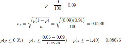
pnorm(-1.40)
## [1] 0.08075666
Thus, there is nearly a 0.081 probability that this bad shipment will sneak in as good. It should be clear that by increasing the sample size n, the inspector can reduce the probability of accepting a shipment with too many defective components. The downside to testing large samples, however, is that it is expensive and time- consuming to test large numbers of items.