Statistics with R
Student Resources
Chapter 1: Introduction and R Instructions
1. Using R, answer the following questions.
(a) The sum of 137 and 242.
Answer:
137 + 242
## [1] 379
(b) The difference between 1,206 and 373.
Answer:
1206 - 373
## [1] 833
(c) The product of 547 and 23.
Answer:
547 * 23
## [1] 12581
(d) Divide 8,840 by 17.
Answer:
8840 / 17
## [1] 520
(e) Raise 11 to the 3rd power.
Answer:
11 ^ 3
## [1] 1331
(f) Find the square root of 64.
Answer:
sqrt(64)
## [1] 8
(g) Find the cube root of 8,000.
Answer:
8000 ^ (1/3)
## [1] 20
In later chapters, we introduce many additional R commands that are highly useful whenever we wish to perform computations.
2. Enter the following small data set directly into the R Workspace, and name it E1_1: 81, 17, 7, 55, 2, 98, 71, 47, 19, 8, 3, 10, 28, 65, 80. Check to make sure that E1_1 contains these elements, and answer the following questions.
#Comment1. Use the c() function to create object E1_1.
E1_1 <- c(81, 17, 7, 55, 2, 98, 71, 47, 19, 8, 3, 10, 28, 65, 80)
#Comment2. Examine contents of E1_1.
E1_1
## [1] 81 17 7 55 2 98 71 47 19 8 3 10 28 65 80
Answer:
#Comment1. Create the object E1_1.
E1_1 <- c(81, 17, 7, 55, 2, 98, 71, 47, 19, 8, 3, 10, 28, 65, 80)
#Comment2. Use the sort() function to rank order data;
#name (i.e., recycle) result E1_1.
E1_1 <- sort(E1_1)
#Comment3. Examine contents of E1_1. Note: the middle value
(or #median) is 28.
E1_1
## [1] 2 3 7 8 10 17 19 28 47 55 65 71 80 81 98
#Comment4. Use the median() function to find median of E1_1.
median(E1_1)
## [1] 28
In the following chapters, we will learn many other R functions that help us perform basic data management and statistical analysis.
(b) Using the max() and min() functions, find the maximum and minimum values of E1_1. Also, using the sum() and mean() functions, find the sum of all the data values as well as the mean of E1_1.
Answer:
#Comment1. Use the min() function to find minimum value in E1_1.
min(E1_1)
## [1] 2
#Comment2. Use the max() function to find maximum value in E1_1.
max(E1_1)
## [1] 98
#Comment3. Use the sum() function to find sum of values in E1_1.
sum(E1_1)
## [1] 591
#Comment4. Use the mean() function to find the mean of E1_1.
mean(E1_1)
## [1] 39.4
(c) Count the number of data values in E1_1. Although it is clear that there are 15 elements, the length() function can be used when we want to know the number of elements contained in data sets of unknown size.
Answer:
#Comment. Use length() function to find number of data items.
#in E1_1.
length(E1_1)
## [1] 15
3. Use the sum() and length() functions to calculate the mean of E1 1.
Answer:
#Comment1. Use ratio of sum() and length(); name the result mean.
mean <- sum(E1_1) / length(E1_1)
#Comment2. Examine contents of mean.
mean
## [1] 39.4
As we see, the mean is the same regardless if we derive it this way, or use mean() to provide the answer more directly. This exercise is included only to provide a little practice writing basic R code; we would normally use the easier approach, mean().
4. R contains a number of built-in data sets that are available for beginning programmers to work on. (To see a list of these free data sets, simply enter data()) at the R prompt in the Console.) For example, one of the data sets is named LakeHuron (named after the Great Lake situated on the Canadian-US border). To learn a bit about this data set, enter at the R prompt ?LakeHuron. When we do this, a page opens to describe the data set, informing us that the LakeHuron data consists of "Annual Measurements of the level, in feet, of Lake Huron, 1875 - 1972." The following questions concern the the LakeHuron data set.
- Use function head(LakeHuron,3) to examine the first three elements of data set LakeHuron. (Use function head(LakeHuron,n) to display the first n data items.)
- Are any data missing? Use function length(LakeHuron).
- What is the lowest level (in feet) of Lake Huron during the 1875-1972 period?
- What is the highest level of Lake Huron during the same period?
- What is the mean level of Lake Huron during this period?
- What is the median level?
#Comment1. Use head() function to view the first three observations.
head(LakeHuron, 3)
## [1] 580.38 581.86 580.97
#Comment2. Does the data set contain one measurement for each year
#from 1875 to 1972, or does it include any missing data values or
#years? (Since there are 98 years from 1875 to 1972, there should be
#98 elements in LakeHuron if there are no missing data.)
length(LakeHuron)
## [1] 98
#Comment3. Use function min() to find lowest level of LakeHuron.
min(LakeHuron)
## [1] 575.96
#Comment4. Use function max() for the highest level of LakeHuron.
max(LakeHuron)
## [1] 581.86
#Comment5. Use function mean() to find mean.
mean(LakeHuron)
## [1] 579.0041
#Comment6. Use function median() to find median.
median(LakeHuron)
## [1] 579.12
Answer: There are no missing data items; all 98 years have a measurement. The minimum and maximum levels are 576 and 581.9 feet, respectively. The mean is 579 feet, the median 579.1.
5. Are the Lake Huron data cross-sectional or longitudinal? How are the data scaled? (That is, are they nominal-scaled, ordinal-scaled, etc.?)
Answer: The Lake Huron data are longitudinal (not cross-sectional) and ratio-scaled.
6. Is there any way that we might be able to use R to provide a picture of the data? Although we have some idea of how the data are distributed (the lowest level is 576, the highest is 581.9, and the mean is 579) a picture can be worth a thousand words.
Answer: We can use the hist() function to create a histogram of the data.
#Comment. Use hist() function to provide histogram; set color blue.
hist(LakeHuron, col = 'blue')
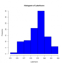
The histogram provides a bit more insight into how the data values are distributed. In fact, the data seem to be distributed normally (that is, somewhat bell-shaped) around the mean of 579 although pulled, or skewed, just slightly to the left.
7. We note that a simple histogram provides a visual glimpse into how data are distributed. Since we have heard about the normal bell-curve distribution, is it possible to see a histogram of that?
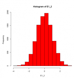
Answer: We can use the rnorm(N) function to generate a set of N normally-distributed data values. (This is a function that we use again in later chapters.) Once we have generated the data and assigned them to an object, we use the hist() function to create a histogram.
#Comment1. Use function rnorm(10000) to generate 10,000
#normally-distributed data values; name the result E1_2.
E1_2 <- rnorm(10000)
#Comment2. Use function hist() to provide histogram; set color red.
hist(E1_2, col = 'red')
8. Should we be very confident that these data really are good representations of the actual water level of Lake Huron over the period from 1875 to 1972? What might be uncontrolled influences on the measurements that are taken each year?
Answer: The times and dates on which the measurements are taken would be important. From one measurement to the next, are there any differences in tides? Have any measurements been taken during different seasons of the year? For example, during the spring the water level would presumably be higher (because of run-off of melting snow and heavy spring precipiation) than during the fall (after a hot summer of evaporation). Also, are the measurements being taken from exactly the same location, presumably somewhere near the middle of the Lake? It is possible that there is no record of where the measurements were taken, especially in the earlier years? The point is that we must always be skeptical of (and raise questions about) the quality of our data before we are in a position to draw sound conclusions from it.
9. Create a data frame consisting of the world's seven largest nations measured on three variables: population, GDP, and percent urban population. (Use Table 1.) Name the data frame E1_3; name the variables Nation, Population, GDP, and Percent Urban. Do not include the other variables.
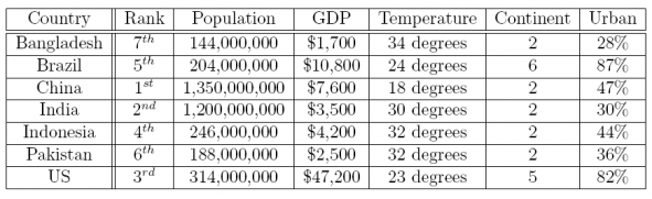
Table 1: Profiles of the World's Seven Most Populous Countries
Answer:
#Comment1. The options(scipen = 999) function overrides the R
#default of reporting very large (and very small) numbers (such
#as the population) in scientific notation.
options(scipen = 999)
#Comment2. Create a vector consisting of the country names; assign
#the result to the object named var1. Note: names are contained in
#quotes (can be either single or double)
var1 <- c( 'Bangalesh', 'Brazil', 'China', 'India', 'Indonesia', 'Pakistan', 'US')
#Comment3. Create a vector consisting of the national populations;
#assign the result to the object named var2.
var2 <- c(144000000, 204000000, 1350000000, 1200000000, 246000000,
188000000, 314000000)
#Comment4. Create a vector consisting of the national GDP; assign
#the result to the object named var3.
var3 <- c(1700, 10800, 7600, 3500, 4200, 2500, 47200)
#Comment5. Create a vector consisting of the percent of nation's
#population living in an urban area; assign result to object var4.
var4 <- c(28, 87, 47, 30, 44, 36, 82)
#Comment6. Create a data frame containing the four objects: var1,
#var2, var3, and var4; assign the result to object E1_3.
E1_3 <- data.frame(Nation = var1, Population = var2, GDP = var3, PercentUrban = var4 )
#Comment7. Review the contents of the data frame E1_3.
E1_3
## Nation Population GDP PercentUrban
## 1 Bangalesh 144000000 1700 28
## 2 Brazil 204000000 10800 87
## 3 China 1350000000 7600 47
## 4 India 1200000000 3500 30
## 5 Indonesia 246000000 4200 44
## 6 Pakistan 188000000 2500 36
## 7 US 314000000 47200 82
10. Answer the following questions concerning the data frame E1_3.
(a) Find the summary statistics (the mean, the median, the maximum, the minimum, the first and third quartiles) of the variable Population.
Answer:
summary(E1_3$Population)
## Min. 1st Qu. Median Mean 3rd Qu. Max.
## 144000000 196000000 246000000 520900000 757000000 1350000000
(b) Find the summary statistics (the mean, the median, the maximum, the minimum, the first and third quartiles) of the variable GDP.
Answer:
summary(E1_3$GDP)
## Min. 1st Qu. Median Mean 3rd Qu. Max.
## 1700 3000 4200 11070 9200 47200
(c) Find the summary statistics (the mean, the median, the maximum, the minimum, the first and third quartiles) of the variable Percent Urban.
Answer:
summary(E1_3$PercentUrban)
## Min. 1st Qu. Median Mean 3rd Qu. Max.
## 28.00 33.00 44.00 50.57 64.50 87.00