Statistics with R
Student Resources
Chapter 8: Confidence Interval Estimation
1. Suppose a random sample of size n = 100 has been selected and the sample mean is found to be x̄ = 67. The population standard deviation is assumed to be σ = 12. Please answer the following questions.
(a) What is the standard error of the mean σx̄?
Answer: 1.2
![]()
(b) What is the margin of error if the confidence level is (1 – α ) = 0.95?
Answer: 2.352
If (1 –α ) = 0.95, then zα/2 =2 = z0.025 = 1.96
qnorm(0.025, lower.tail = FALSE) * 12 / sqrt(100)
## [1] 2.351957
Therefore, zα/2σx̄ = (1.96)(1.2) = 2.352
(c) What is the 95% confidence interval estimate of µ?
Answer: 67 ± 2.352 or [64.648, 69.352]
x̄ ± zα/2σx̄
67 ± 2.352
[64.648, 69.352]
#Comment1. To find the upper bound of the confidence interval
#estimate, add the margin of error to the sample mean.
67 + qnorm(0.025, lower.tail = FALSE) * 12 / sqrt(100)
## [1] 69.35196
#Comment2. To find the lower bound of the confidence interval
#estimate, subtract the margin of error to the sample mean.
67 - qnorm(0.025, lower.tail = FALSE) * 12 / sqrt(100)
## [1] 64.64804
2. Suppose a random sample of size n = 36 has been selected from a population with σ = 30 and a sample mean of x̄ = 205
(a) What is the 90% confidence interval estimate of µ ?
Answer: 205 ± 8.225
If (1 – α ) = 0.90, then zα/2 =2 = z0:050 = 1.645, then
qnorm(0.05, lower.tail = FALSE)
## [1] 1.644854
x̄ ± zα/2σx̄
![]()
205 ± 8.225
[196.775, 213.225]
#Comment1. To find the upper bound of the confidence interval
#estimate, add the margin of error to the sample mean
205 + qnorm(0.05, lower.tail = FALSE) * 30 / sqrt(36)
## [1] 213.2243
#Comment2. To find the lower bound of the confidence interval
#estimate, subtract the margin of error to the sample mean.
205 - qnorm(0.05, lower.tail = FALSE) * 30 / sqrt(36)
## [1] 196.7757
(b) What is the 95% confidence interval estimate of µ?
Answer: 205 ± 9.80
If (1 – α ) = 0.95, then zα/2 = z0.025 = 1.96, then
qnorm(0.025, lower.tail = FALSE)
## [1] 1.959964
x̄ ± zα/2σx̄
![]()
205 ± 9.80
[195:20; 214:80]
#Comment1. To find the upper bound of the confidence interval
#estimate, add the margin of error to the sample mean.
205 + qnorm(0.025, lower.tail = FALSE) * 30 / sqrt(36)
## [1] 214.7998
#Comment2. To find the lower bound of the confidence interval
#estimate, subtract the margin of error to the sample mean.
205 - qnorm(0.025, lower.tail = FALSE) * 30 / sqrt(36)
## [1] 195.2002
(c) What is the 99% confidence interval estimate of µ ?
Answer: 205 ± 12.880
If (1 – α ) = 0.99, then zα/2 = z0.005 = 2.576, then
qnorm(0.005, lower.tail = FALSE)
## [1] 2.575829
x̄ ± zα/2σx̄
![]()
205 ± 12.880
[192.12, 217.88]
#Comment1. To find the upper bound of the confidence interval
#estimate, add the margin of error to the sample mean.
205 + qnorm(0.005, lower.tail = FALSE) * 30 / sqrt(36)
## [1] 217.8791
#Comment2. To find the lower bound of the confidence interval
#estimate, subtract the margin of error to the sample mean.
205 - qnorm(0.005, lower.tail = FALSE) * 30 / sqrt(36)
## [1] 192.1209
3. If a 99% confidence interval is [228, 232] for a population with σ = 10, what is n?
Answer: n = 166
Margin of error=(232 – 228)/2 = 2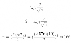
qnorm(0.005, lower.tail = FALSE)
## [1] 2.575829
Checking the margin of error when n = 166, (1 –α ) = 0.99, and σ= 10

4. Provide the interval estimate at the 90% confidence level for each case below.
(a) For n = 40, the sample mean is x̄ = 70; assume it is known that σ = 6.
Answer: 70 ± 1.56

70 ± 1.56
[68.44, 71.56]
#Comment1. To find the upper bound of the confidence interval
#estimate, add the margin of error to the sample mean.
70 + qnorm(0.05, lower.tail = FALSE) * 6 / sqrt(40)
## [1] 71.56045
#Comment2. To find the lower bound of the confidence interval
#estimate, subtract the margin of error to the sample mean.
70 - qnorm(0.05, lower.tail = FALSE) * 6 / sqrt(40)
## [1] 68.43955
(b) For n = 120, the sample mean is x̄ = 44; assume it is known that σ = 2.
Answer: 44 ± 0.30
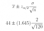
44 ± 0.30
[43.70, 44.30]
#Comment1. To find the upper bound of the confidence interval
#estimate, add the margin of error to the sample mean.
44 + qnorm(0.05, lower.tail = FALSE) * 2 / sqrt(120)
## [1] 44.30031
#Comment2. To find the lower bound of the confidence interval
#estimate, subtract the margin of error to the sample mean.
44 - qnorm(0.05, lower.tail = FALSE) * 2 / sqrt(120)
## [1] 43.69969
(c) For n = 81, the sample mean is x̄ = 0; assume it is known that σ= 9.
Answer: 0 ± 1.645
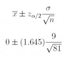
0 ± 1.645
[–1:645; 1:645]
#Comment1. To find the upper bound of the confidence interval
#estimate, add the margin of error to the sample mean.
0 + qnorm(0.05, lower.tail = FALSE) * 9 / sqrt(81)
## [1] 1.644854
#Comment2. To find the lower bound of the confidence interval
#estimate, subtract the margin of error to the sample mean.
0 - qnorm(0.05, lower.tail = FALSE) * 9 / sqrt(81)
## [1] -1.644854
(d) For n = 30, the sample mean is x̄ = –12; assume it is known that σ = 7.
Answer: –12 ± 2.10
![]()
![]()
–12 ± 2.10
[–14.10, –9.90]
#Comment1. To find the upper bound of the confidence interval
#estimate, add the margin of error to the sample mean.
-12 + qnorm(0.05, lower.tail = FALSE) * 7 / sqrt(30)
## [1] -9.897845
#Comment2. To find the lower bound of the confidence interval
#estimate, subtract the margin of error to the sample mean.
-12 - qnorm(0.05, lower.tail = FALSE) * 7 / sqrt(30)
## [1] -14.10215
5. In a continuing study of the amount MBA students are spending each term on text- books, data were collected on n = 81 students. In previous studies, the population standard deviation has been σ = $24.
(a) What is the margin of error at the 99% confidence level?
Answer: 6.87
qnorm(0.005, lower.tail = FALSE) * 24 / sqrt(81)
## [1] 6.868878

(b) If the mean from the most recent sample was x̄ = $288, what is the 99% confidence interval estimate of the population mean µ ?
Answer: $288 ± $6.87
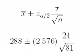
288 ± 6.87
[281, 295]
#Comment1. To find the upper bound of the confidence interval
#estimate, add the margin of error to the sample mean.
288 + qnorm(0.005, lower.tail = FALSE) * 24 / sqrt(81)
## [1] 294.8689
#Comment2. To find the lower bound of the confidence interval
#estimate, subtract the margin of error to the sample mean.
288 - qnorm(0.005, lower.tail = FALSE) * 24 / sqrt(81)
## [1] 281.1311
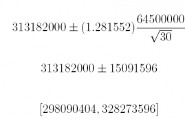
6. Assume that the average financial endowment of U.S. universities is $313,182, 000. If this estimate is developed on a random sample size of n = 30, what is the 80% confidence interval estimate of the population mean ? Assume the population standard deviation is σ = $64, 500, 000.
Answer: $313, 182, 000 ± $15, 091, 596
(1 –α ) = 0.80
zα/2 = z0.10 = 1.281552
#Comment1. Value of z providing an area of 0.10 in upper tail.
qnorm(0.10, lower.tail = FALSE)
## [1] 1.281552
#Comment2. Margin of error.
qnorm(0.10, lower.tail = FALSE) * 64500000 / sqrt(30)
## [1] 15091596

#Comment1. To find the upper bound of the confidence interval
#estimate, add the margin of error to the sample mean.
313182000 + qnorm(0.10, lower.tail = FALSE) * 64500000 / sqrt(30)
## [1] 328273596
#Comment2. To find the lower bound of the confidence interval
#estimate, subtract the margin of error to the sample mean.
313182000 - qnorm(0.10, lower.tail = FALSE) * 64500000 / sqrt(30)
## [1] 298090404
7. Referring to the previous exercise, if the data tend to be highly skewed because of the presence of a dozen or so very wealthy universities, does the above procedure lead to reliable estimates? If not, comment on what might be done to improve the estimation procedure.
Answer: If the size of the data set is n = 30, the sampling distribution of x̄ usually approaches normal. However, when the data are highly skewed, it is a good practice to increase the size of the data set, perhaps to something as high as n = 60, if possible. In this, we make it very likely that the sampling distribution of x̄ approaches normal.
8. Find the following probabilities using the t distribution with n = 23.
(a) What is the probability that t will be greater than or equal to 0? That is, what is p(t ≥ 0, df = 23 – 1 = 22)?
Answer: 0.5000
#Comment1. 1 minus probability t is less than or equal to 0.
1 - pt(0, 22)
## [1] 0.5
#Comment2. Or using the "lower.tail=FALSE" argument.
pt(0, 22, lower.tail = FALSE)
## [1] 0.5
(b) What is the probability that t will be greater than or equal to 2.074? That is, what is p(t ≥ 2.074, df = 23 – 1 = 22)?
Answer: 0.02499
#Comment1. 1 minus probability t is less than or equal to 2.074.
1 - pt(2.074, 22)
## [1] 0.02499358
#Comment2. Or using the "lower.tail=FALSE" argument.
pt(2.074, 22, lower.tail = FALSE)
## [1] 0.02499358
(c) What is the probability that t will be less than or equal to 2.819? That is, what is p(t ≤ 2.819, df = 23 – 1 = 22)?
Answer: 0.995
#Comment. Probability t is less than or equal to 2.819.
pt(2.819, 22)
## [1] 0.9950028
(d) What is the probability that t will be less than or equal to -1.321? That is, what is p(t ≤ 1.321, df = 23 – 1 = 22)?
Answer: 0.10
#Comment. Probability t is less than or equal to -1.321.
pt(-1.321, 22)
## [1] 0.1000388
(e) What is the probability t will fall between -0.858 and 1.717? That is, what is the p(–0.858 ≤ t ≤ 1.717)?
Answer: 0.7499
#Comment. Subtract pt(-0.858,22) from pt(1.717,22).
pt(1.717, 22) - pt(-0.858, 22)
## [1] 0.7499147
(f) What is the probability t will fall between -1.717 and -0.858? That is, what is the p(–1.717≤ t ≤ 0.858)?
Answer: 0.1501
#Comment. Subtract pt(-1.717,22) from pt(-0.858,22).
pt(-0.858, 22) - pt(-1.717, 22)
## [1] 0.1500585
9. Find the value for t for each of the following questions.
(a) What is the value of t which has an area to its right of 0.05 when the sample size is n = 28.
Answer: 1.703
#Comment1. Value of t cutting off area to its left of 0.95.
qt(0.95, 27)
## [1] 1.703288
#Comment2. Include the "lower.tail=FALSE" argument.
qt(0.05, 27, lower.tail = FALSE)
## [1] 1.703288
(b) What is the value of t which has an area to its right of 0.025 when the sample size is n = 41.
Answer: 2.021
#Comment1. Value of t cutting off area to its left of 0.975.
qt(0.975, 40)
## [1] 2.021075
#Comment2. Include the "lower.tail=FALSE" argument.
qt(0.025, 40, lower.tail = FALSE )
## [1] 2.021075
(c) What is the value of t which has an area to its right of 0.500 when the sample size is n = 11.
Answer: 0.000
#Comment. Value of t cutting off area to its left of 0.5000.
qt(0.5000, 10)
## [1] 0
(d) What is the value of t which has an area to its left of 0.01 when the sample size is n = 76.
Answer: -2.377
#Comment. Value of t cutting off area to its left of 0.01.
qt(0.01, 75)
## [1] -2.377102
(e) What is the value of t which has an area to its left of 0.10 when the sample size is n = 33.
Answer: -1.309
#Comment. Value of t cutting off area to its left of 0.10.
qt(0.10, 32)
## [1] -1.308573
(f) What is the value of t which has an area to its left of 0.20 when the sample size is n = 100.
Answer: -0.8453
#Comment. Value of t cutting off area to its left of 0.20.
qt(0.20, 99)
## [1] -0.845267
10. A sample of gasoline prices was taken at n = 70 service stations across the U.S., and the sample mean price per gallon was found to be x̄ = $3.67, the sample standard deviation s = $0.21.
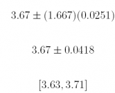
(a) What is the 90% confidence interval estimate of the population mean price per gallon µ?
Answer: 3.67 ± 0.0418
![]()
#Comment1. The value of t providing area of 0.05 in upper tail.
qt(0.05, 69, lower.tail = FALSE)
## [1] 1.667239
#Comment2. The margin of error.
qt(0.05, 69, lower.tail = FALSE) * 0.21 / sqrt(70)
## [1] 0.04184736
#Comment1. To find the upper bound of the confidence interval
#estimate, add the margin of error to the sample mean.
3.67 + qt(0.05, 69, lower.tail = FALSE) * 0.21 / sqrt(70)
## [1] 3.711847
#Comment2. To find the lower bound of the confidence interval
#estimate, subtract the margin of error to the sample mean.
3.67 - qt(0.05, 69, lower.tail = FALSE) * 0.21 / sqrt(70)
## [1] 3.628153
(b) What is the 95% confidence interval estimate of the population mean price per gallon µ?
Answer: 3.67± 0.0501
![]()
#Comment1. The value of t providing area of 0.025 in upper tail.
qt(0.025, 69, lower.tail = FALSE)
## [1] 1.994945
#Comment2. The margin of error.
qt(0.025, 69, lower.tail = FALSE) * 0.21 / sqrt(70)
## [1] 0.05007273
3.67 ± (1.995)(0.0251)
3.67 ± 0.0501
[3.62, 3.72]
#Comment1. To find the upper bound of the confidence interval
#estimate, add the margin of error to the sample mean.
3.67 + qt(0.025, 69, lower.tail = FALSE) * 0.21 / sqrt(70)
## [1] 3.720073
#Comment2. To find the lower bound of the confidence interval
#estimate, subtract the margin of error to the sample mean.
3.67 - qt(0.025, 69, lower.tail = FALSE) * 0.21 / sqrt(70)
## [1] 3.619927
(c) What is the 99% confidence interval estimate of the population mean price per gallon µ?
Answer: 3.67± 0.0665

#Comment1. The value of t providing area of 0.005 in upper tail.
qt(0.005, 69, lower.tail = FALSE)
## [1] 2.648977
#Comment2. The margin of error.
qt(0.005, 69, lower.tail = FALSE) * 0.21 / sqrt(70)
## [1] 0.06648879
3.67 ± (2.649)(0.0251)
3.67 ± 0.0665
[3.60, 3.74]
#Comment1. To find the upper bound of the confidence interval
#estimate, add the margin of error to the sample mean.
3.67 + qt(0.005, 69, lower.tail = FALSE) * 0.21 / sqrt(70)
## [1] 3.736489
#Comment2. To find the lower bound of the confidence interval
#estimate, subtract the margin of error to the sample mean.
3.67 - qt(0.005, 69, lower.tail = FALSE) * 0.21 / sqrt(70)
## [1] 3.603511
11. A survey finds that the average British household is expected to spend £868 on holiday-related expenses during the next Christmas period. This amount covers not only gifts, but food, beverages, and decorations. Assume the study is based on n = 94 randomly sampled households throughout the U.K. Assume that the sample standard deviation is s=£162.
(a) What is the 60% confidence interval estimate of the population mean amount- to-be-spent µ during the 2013 Christmas holiday period?
Answer: £868 ± £14.13

#Comment1. The value of t providing area of 0.20 in upper tail.
qt(0.20, 93, lower.tail = FALSE)
## [1] 0.8455033
#Comment2. The margin of error.
qt(0.20, 93, lower.tail = FALSE) * 162 / sqrt(94)
## [1] 14.12753
868± 14.13
[854, 882]
#Comment1. To find the upper bound of the confidence interval
#estimate, add the margin of error to the sample mean.
868 + qt(0.20, 93, lower.tail = FALSE) * 162 / sqrt(94)
## [1] 882.1275
#Comment2. To find the lower bound of the confidence interval
#estimate, subtract the margin of error to the sample mean.
868 - qt(0.20, 93, lower.tail = FALSE) * 162 / sqrt(94)
## [1] 853.8725
(b) What is the 80% confidence interval estimate of the population mean amount- to-be-spent µ during the next Christmas holiday period?
Answer: £868 ± £21.57

#Comment1. The value of t providing area of 0.10 in upper tail.
qt(0.10, 93, lower.tail = FALSE)
## [1] 1.290721
#Comment2. The margin of error.
qt(0.10, 93, lower.tail = FALSE) * 162 / sqrt(94)
## [1] 21.56669
868 ± (1.291)(16.71)
868 ± 21.57
[846, 890]
#Comment1. To find the upper bound of the confidence interval
#estimate, add the margin of error to the sample mean.
868 + qt(0.10, 93, lower.tail = FALSE) * 162 / sqrt(94)
## [1] 889.5667
#Comment2. To find the lower bound of the confidence interval
#estimate, subtract the margin of error to the sample mean.
868 - qt(0.10, 93, lower.tail = FALSE) * 162 / sqrt(94)
## [1] 846.4333
(c) What is the 90% confidence interval estimate of the population mean amount- to-be-spent µ during the next Christmas holiday period?
Answer: £868 ± £27.76

#Comment1. The value of t providing area of 0.05 in upper tail.
qt(0.05, 93, lower.tail = FALSE)
## [1] 1.661404
#Comment2. The margin of error.
qt(0.05, 93, lower.tail = FALSE) * 162 / sqrt(94)
## [1] 27.76043
868 ± (1.661)(16.71)
868 ± 27.76
[840, 896]
#Comment1. To find the upper bound of the confidence interval
#estimate, add the margin of error to the sample mean.
868 + qt(0.05, 93, lower.tail = FALSE) * 162 / sqrt(94)
## [1] 895.7604
#Comment2. To find the lower bound of the confidence interval
#estimate, subtract the margin of error to the sample mean.
868 - qt(0.05, 93, lower.tail = FALSE) * 162 / sqrt(94)
## [1] 840.2396
12. Accordingly to one of the 2016 U.S. Presidential candidates, the average net wealth of those individuals classi ed as members of the (upper) 1% is $8, 400, 000. If this value was developed on a sample of size n = 20 individuals, can you see any problem using the con dence interval estimate methods of Chapter 8?
Answer: Ideally, with such a small sample, we want the underlying population distribution itself to be normally distributed. In that way, we could safely use the confidence interval estimation methods of Chapter 8. If the underlying distribution is merely symmetric about the mean, we could probably use these methods. However, like income and property values, net wealth tends to be skewed to the
greater values. Accordingly, the best course of action is to collect a larger sample size: n = 30 might be suffcient; n ≥ 50 would be better still.
13. The cafe_ratings data (available on the companion website) consist of a sample of n = 50 highly-rated restaurants in a certain U.S. city; the variables include cuisine (for type of cuisine: American, Chinese, French, Italian, and Japanese), rating (for the rating on a 30-point scale), and price (for the average price of a meal). As a first step, import cafe_ratings into the object E8_1. Use R to provide answers.
(a) What are the point estimates of the mean and standard deviation of price µ?
Answer: the sample mean is $93.46, the sample standard deviation is $75.65.
#Comment1. Import the cafe_ratings data into the object E8_1.
E8_1 <- cafe_ratings
#Comment2. Identify the variable names.
names(E8_1)
## [1] "cuisine" "price" "rating"
#Comment3. Use mean() to find mean of price.
mean(E8_1$price)
## [1] 93.46
#Comment4. Use sd() to find the standard deviation of price.
sd(E8_1$price)
## [1] 75.64935
(b) What is the margin of error at the 95% level of confidence?
Answer: $21.50
qt(0.025, 49, lower.tail = FALSE) * sd(E8_1$price) /
sqrt(length(E8_1$price))
## [1] 21.49931
(c) Find the 95% confidence interval estimate of the population mean µ.
Answer: The 95% confidence interval estimate is [$71.96, $114.96].
#Comment1. For the upper bound of the interval estimate, add
#the margin of error to the sample mean of E8_1.
mean(E8_1$price) + qt(0.025, 49, lower.tail = FALSE) *
sd(E8_1$price) / sqrt(length(E8_1$price))
## [1] 114.9593
#Comment2. For the lower bound of the interval estimate,
#subtract the margin of error from the sample mean of E8_1.
mean(E8_1$price) - qt(0.025, 49, lower.tail = FALSE) *
sd(E8_1$price) / sqrt(length(E8_1$price))
## [1] 71.96069
14. Referring to the preceding exercise, find the 95% confidence interval estimate using the t.test() function. Does the answer using this approach square with the answer in the preceding exercise?
Answer: Yes, it does. The 95% confidence interval estimate is [$71.96, $114.96].
#Comment. t.test() gives 95% interval estimate of mean.
t.test(E8_1$price, conf = 0.95)
##
## One Sample t-test
##
## data: E8_1$price
## t = 8.7359, df = 49, p-value = 1.465e-11
## alternative hypothesis: true mean is not equal to 0
## 95 percent confidence interval:
## 71.96069 114.95931
## sample estimates:
## mean of x
## 93.46
15. Find the 90% confidence interval estimate of price from the cafe_ratings data set. Use both methods.
Answer: Both methods produce the same 90% confidence interval: [$75.52, $111.40].
#Comment1. For the upper bound of the interval estimate, add
#the margin of error to the sample mean of E8_1.
mean(E8_1$price) + qt(0.05, 49, lower.tail = FALSE) *
sd(E8_1$price) / sqrt(length(E8_1$price))
## [1] 111.3965
#Comment2. For the lower bound of the interval estimate,
#subtract the margin of error from the sample mean of E8_1.
mean(E8_1$price) - qt(0.05, 49, lower.tail = FALSE) *
sd(E8_1$price) / sqrt(length(E8_1$price))
## [1] 75.52353
#Comment3. Use the t.test() function for the 90% interval estimate.
t.test(E8_1$price, conf = 0.90)
##
## One Sample t-test
##
## data: E8_1$price
## t = 8.7359, df = 49, p-value = 1.465e-11
## alternative hypothesis: true mean is not equal to 0
## 90 percent confidence interval:
## 75.52353 111.39647
## sample estimates:
## mean of x
## 93.46
16. Find the 99% confidence interval estimate of price from the cafe_ratings data set. Use both methods.
Answer: Both methods produce the same 99% confidence interval: [$64.79, $122.13].
#Comment1. For the upper bound of the interval estimate, add
#the margin of error to the sample mean of E8_1.
mean(E8_1$price) + qt(0.005, 49, lower.tail = FALSE) *
sd(E8_1$price) / sqrt(length(E8_1$price))
## [1] 122.1313
#Comment2. For the lower bound of the interval estimate,
#subtract the margin of error from the sample mean of E8_1.
mean(E8_1$price) - qt(0.005, 49, lower.tail = FALSE) *
sd(E8_1$price) / sqrt(length(E8_1$price))
## [1] 64.78871
#Comment3. Use the t.test() function for the 99% interval estimate.
t.test(E8_1$price, conf = 0.99)
##
## One Sample t-test
##
## data: E8_1$price
## t = 8.7359, df = 49, p-value = 1.465e-11
## alternative hypothesis: true mean is not equal to 0
## 99 percent confidence interval:
## 64.78871 122.13129
## sample estimates:
## mean of x
## 93.46
17. The director of the Office of Research Support at a major U.S. research university wanted to get an idea of the amount being spent on dining by faculty attending academic conferences over the course of a year. Accordingly, she directed her staff to randomly sample the annual expense reimbursement reports from 100 faculty members during 2016. Read the dining data (from the companion website) into
the object named E8_2. Find the 90% confidence interval estimate of .
Answer: The 90% confidence interval estimate of is [$891.25, $947.45].
#Comment1. Read dining data into the object named E8_2.
E8_2 <- dining
#Comment2. Identify the variable name using the names() function.
names(E8_2)
## [1] "annual.cost"
#Comment3. Use the t.test() function to find 90% interval estimate.
t.test(E8_2$annual.cost, conf = 0.90)
##
## One Sample t-test
##
## data: E8_2$annual.cost
## t = 54.326, df = 99, p-value < 2.2e-16
## alternative hypothesis: true mean is not equal to 0
## 90 percent confidence interval:
## 891.2516 947.4484
## sample estimates:
## mean of x
## 919.35
18. The manager of an insurance office wished to gain a better understanding of the dollar value of the newly-purchased automobiles his rm had insured over the previous 12 months. To this end, he randomly selected 70 insurance applications from the previous year that listed the total cost of each vehicle insured, including market value, taxes, and licensing fees. Using the insurance data (from the companion website), nd the 99% confidence interval estimate of µ. As a first step, read the insurance data into the object E8_3.
Answer: The 99% confidence interval estimate of is [$16087, $21161].
#Comment1. Read insurance data into the object named E8_3.
E8_3 <- insurance
#Comment2. Identify the variable name.
names(E8_3)
## [1] "automobile"
#Comment3. Use the t.test() function to find 99% interval estimate.
t.test(E8_3$automobile, conf = 0.99)
##
## One Sample t-test
##
## data: E8_3$automobile
## t = 19.443, df = 69, p-value < 2.2e-16
## alternative hypothesis: true mean is not equal to 0
## 99 percent confidence interval:
## 16086.66 21161.34
## sample estimates:
## mean of x
## 18624
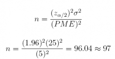
19. What sample size n is required to provide a margin of error of 5 at the 95% confidence level. Assume the population standard deviation is σ = 25.
Answer: n = 97
qnorm(0.025, lower.tail = FALSE)
## [1] 1.959964
(qnorm(0.025, lower.tail = FALSE) * 25 / 5) ^ 2
## [1] 96.03647
check:
![]()
qnorm(0.025, lower.tail = FALSE) * 25 / sqrt(97)
## [1] 4.975105
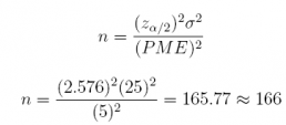
20. What sample size n is required to provide a margin of error of 5 at the 99% confidence level. Assume the population standard deviation is σ = 25.
Answer: n = 166
qnorm(0.005, lower.tail = FALSE)
## [1] 2.575829
(qnorm(0.005, lower.tail = FALSE) * 25 / 5) ^ 2
## [1] 165.8724
check:
![]()
qnorm(0.005, lower.tail = FALSE) * 25 / sqrt(166)
## [1] 4.998078
21. Suppose the Dean of a large medical college wishes to estimate the mean student age of the most recent entering class of aspiring physicians pursuing an M.D. degree. A quick pilot study reveals that 3 years might be used as an estimate of the value of σ. If a 95% confidence interval estimate with a margin of error 1 is desired, what sample size should we recommend?
Answer: n = 35

qnorm(0.025, lower.tail = FALSE)
## [1] 1.959964
(qnorm(0.025, lower.tail = FALSE) * 3 / 1) ^ 2
## [1] 34.57313
check:

qnorm(0.025, lower.tail = FALSE) * 3 / sqrt(35)
## [1] 0.9938831
22. The commute-to-work time for the residents of the world's large cities has been investigated extensively. A pilot study involving a random sample of residents of Toronto is used to provide an estimate of σ= 10 minutes for the population standard deviation.
(a) If we want to estimate the population mean commute-to-work time µ for the residents of Toronto with a margin of error of 2 minutes, what sample size n should we recommend? Assume 90% confidence.
Answer: n = 68
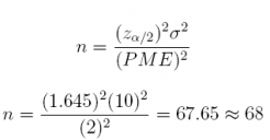
qnorm(0.05, lower.tail = FALSE)
## [1] 1.644854
(qnorm(0.05, lower.tail = FALSE) * 10 / 2) ^ 2
## [1] 67.63859
check:
![]()
qnorm(0.05, lower.tail = FALSE) * 10 / sqrt(68)
## [1] 1.994678
(b) If we want to estimate the population mean commute-to-work time µ for the residents of Toronto with a margin of error of 1 minute, what sample size n should we recommend? Assume 90% confidence.
Answer: n = 271
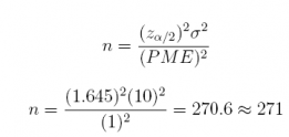
(qnorm(0.05, lower.tail = FALSE) * 10 / 1) ^ 2
## [1] 270.5543
check:
![]()
qnorm(0.05, lower.tail = FALSE) * 10 / sqrt(271)
## [1] 0.9991774
23. A sample of 64 MBA students at the London Business School (LBS) reported they spent an average of £252.45 on textbooks and case materials per semester. Assume the population standard deviation is σ=£74.50.
(a) What is the 95% confidence interval estimate for the mean amount spent µ per term by an MBA student at LBS?
Answer: £252.45 ± £18.25 or [£234.20, £270.70]
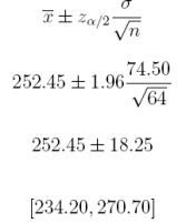
#Comment1. For the lower bound of the interval estimate,
#subtract the margin of error from the sample mean.
252.45 - qnorm(0.025, lower.tail = FALSE) * 74.50 / sqrt(64)
## [1] 234.1978
#Comment2. For the upper bound of the interval estimate, add
#the margin of error to the sample mean.
252.45 + qnorm(0.025, lower.tail = FALSE) * 74.50 / sqrt(64)
## [1] 270.7022
(b) How large a sample would be needed to estimate µ with a margin of error of £10 at 90% confidence?
Answer: n = 151
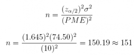
qnorm(0.05, lower.tail = FALSE)
## [1] 1.644854
(qnorm(0.05, lower.tail = FALSE) * 74.50 / 10) ^ 2
## [1] 150.1644
check:
![]()
qnorm(0.05, lower.tail = FALSE) * 74.50 / sqrt(151)
## [1] 9.972294
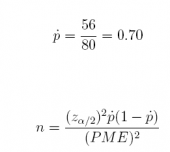
24. In a pilot study, n = 80 respondents have been interviewed, 56 of whom have answered "yes" to a particular survey question. What sample size n is required if we wish to estimate the population proportion p of "yes" answers with a margin of error of 0.02 at the 95% level of confidence?
Answer: n = 2, 017
![]()
qnorm(0.025, lower.tail = FALSE)
## [1] 1.959964
(1.96^2) * (0.70) * (1 - 0.70) / (0.02 ^ 2)
## [1] 2016.84
check:

qnorm(0.025, lower.tail = FALSE) * sqrt((0.70) * (1 - 0.70) / (2017))
## [1] 0.01999884
25. Referring to the previous exercise, what sample size should we recommend if we had no pilot study data to go on? Would n be greater or less than the n recommended in the previous exercise? Assume the study is investigating a question never before researched.
Answer: The sample size should be greater than n = 2, 017 since we would use ṗ = 0.50, the most conservative value when determining sample size. In fact, when ṗ = 0.50, n = 2, 401.
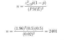
(1.96^2) * (0.50) * (1 - 0.50) / (0.02 ^ 2)
## [1] 2401
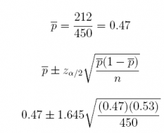
26. In a study of consumer confidence among middle-class Indian families, 450 were interviewed in the metropolitan area Mumbai. When asked about having to cut back on discretionary purchases of big-ticket items, 212 of 450 responded that their families had done so over the previous 6 months.
(a) What is the 90% confidence interval estimate of the population proportion p of this type of household cutting back on discretionary spending?
Answer: 0.47 ± 0.0387
qnorm(0.05, lower.tail = FALSE)
## [1] 1.644854
0.47 ± 0.0387
[0.4313,0.5087]
#Comment1.For the lower bound of the interval estimate,
#subtract the margin of error from the sample proportion.
0.47 - qnorm(0.05, lower.tail = FALSE) * sqrt((0.47) *
(1 - 0.47) / (450))
## [1] 0.4313003
#Comment2. For the upper bound of the interval estimate, add
#the margin of error to the sample proportion.
0.47 + qnorm(0.05, lower.tail = FALSE) * sqrt((0.47) *
(1 - 0.47) / (450))
## [1] 0.5086997
(b) What sample size should we recommend to achieve a margin of error of 0.03?
Answer: n = 749
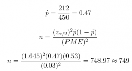
(1.645^2) * (0.47) * (1 - 0.47) / (0.03 ^ 2)
## [1] 748.9676
check:

qnorm(0.05, lower.tail = FALSE) * sqrt((0.47) *
(1 - 0.47) / (749))
## [1] 0.02999668
27. Referring to the previous exercise, answer the following questions.
(a) How large a sample size n would be required to achieve a 99% confidence interval estimate of p with a margin of error of 0.03?
Answer: n=1,837
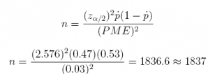
qnorm(0.005, lower.tail = FALSE)
## [1] 2.575829
(2.576^2) * (0.47) * (1 - 0.47) / (0.03 ^ 2)
## [1] 1836.635
check:
![]()
qnorm(0.005, lower.tail = FALSE) * sqrt((0.47) *
(1 - 0.47) / (1837))
## [1] 0.02999503
(b) How large a sample size n would be required to achieve a 99% confidence interval estimate of p with a margin of error of 0.025?
Answer: n = 2, 645
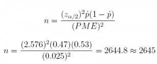
(2.576^2) * (0.47) * (1 - 0.47) / (0.025 ^ 2)
## [1] 2644.755
check:
![]()
qnorm(0.005, lower.tail = FALSE) * sqrt((0.47) *
(1 - 0.47) / (2645))
## [1] 0.02499719
28. A human resources manager at a small university in the U.S. has been considering a change to the structure of employee benefits (in terms of healthcare coverage and pension savings). To get an idea of how receptive faculty, administrators, and staff members might be to the proposed changes, she has decided to conduct a survey in which n = 188 respondents could register their support or opposition. Using the benefits data (from the companion website) to answer the following questions. Note: 0 denotes opposition, 1 support. As a first step, import the benefits data into the object named E8_4 and use the names() function to identify the variable name.
(a) What is the 90% confidence interval estimate of the population proportion p of university employees who favor the change to their benefits package?
Answer: [0.5697, 0.6857]
#Comment1. Import the benefits data into the object E8_4.
E8_4 <- benefits
#Comment2. Find variable name in benefits.
names(E8_4)
## [1] "agree"
#Comment3. Find sample proportion; assign value to object pbar.
pbar <- sum(E8_4$agree) / length(E8_4$agree)
#Comment4. What is the value of pbar, the sample proportion?
pbar
## [1] 0.6276596
#Comment5. For the lower bound of the interval estimate,
#subtract the margin of error from the sample proportion.
pbar - qnorm(0.05, lower.tail = FALSE) * sqrt((pbar) * (1 - pbar)
/ (length(E8_4$agree)))
## [1] 0.5696659
#Comment6. For the upper bound of the interval estimate,
#add the margin of error to the sample proportion.
pbar + qnorm(0.05, lower.tail = FALSE) * sqrt((pbar) * (1 - pbar)
/ (length(E8_4$agree)))
## [1] 0.6856532
(b) What is the 95% confidence interval estimate of the population proportion p of university employees who favor the change to their benefits package?
Answer: [0.5586, 0.6968]
#Comment1. For the lower bound of the interval estimate,
#subtract the margin of error from the sample proportion.
pbar - qnorm(0.025, lower.tail = FALSE) * sqrt((pbar) * (1 - pbar)
/ (length(E8_4$agree)))
## [1] 0.5585559
#Comment2. For the upper bound of the interval estimate,
#add the margin of error to the sample proportion.
pbar + qnorm(0.025, lower.tail = FALSE) * sqrt((pbar) * (1 - pbar)
/ (length(E8_4$agree)))
## [1] 0.6967633
(c) What is the 99% confidence interval estimate of the population proportion p of university employees who favor the change to their benefits package?
Answer: [0.5368, 0.7185]
#Comment1. For the lower bound of the interval estimate,
#subtract the margin of error from the sample proportion.
pbar - qnorm(0.005, lower.tail = FALSE) * sqrt((pbar) * (1 - pbar)
/ (length(E8_4$agree)))
## [1] 0.5368419
#Comment2. For the upper bound of the interval estimate,
#add the margin of error to the sample proportion.
pbar + qnorm(0.005, lower.tail = FALSE) * sqrt((pbar) * (1 - pbar)
/ (length(E8_4$agree)))
## [1] 0.7184772
29. Use the t.test() function to confirm that the confidence interval estimates from the previous exercise (parts (a), (b), and (c)) are correct.
(a) Answer: the 90% confidence interval estimate is [0.5692, 0.6861].
t.test(E8_4$agree, conf.level = 0.90)
##
## One Sample t-test
##
## data: E8_4$agree
## t = 17.755, df = 187, p-value < 2.2e-16
## alternative hypothesis: true mean is not equal to 0
## 90 percent confidence interval:
## 0.5692216 0.6860976
## sample estimates:
## mean of x
## 0.6276596
(b) Answer: the 95% confidence interval estimate is [0.5579, 0.6974].
t.test(E8_4$agree, conf.level = 0.95)
##
## One Sample t-test
##
## data: E8_4$agree
## t = 17.755, df = 187, p-value < 2.2e-16
## alternative hypothesis: true mean is not equal to 0
## 95 percent confidence interval:
## 0.5579200 0.6973991
## sample estimates:
## mean of x
## 0.6276596
(c) Answer: the 99% confidence interval estimate is [0.5357, 0.7197].
t.test(E8_4$agree, conf.level = 0.99)
##
## One Sample t-test
##
## data: E8_4$agree
## t = 17.755, df = 187, p-value < 2.2e-16
## alternative hypothesis: true mean is not equal to 0
## 99 percent confidence interval:
## 0.5356609 0.7196582
## sample estimates:
## mean of x
## 0.6276596
Note that the answers to Exercises 28 and 29 diverge very slightly. But because the magnitude of the difference is so small, we will usually prefer to use the t.text() function when finding confidence interval estimates of the population proportion. While the approach taken in Exercise 28 provides answers that are exactly correct– and moreover the method used gives us a chance to practice our coding skills–it
is easier and quicker to use the t.test() function, particularly because it provides answers that are essentially correct.
