Using Software in Qualitative Research
A Step-by-Step Guide
Student Resources
Chapter 13 – Interrogating Data (NVivo)
Chapter 13 discusses interrogation of data that can happen at varied levels and at many moments during analysis. Already in Chapter 6 we referred to Text search tools where the content is explored. Interrogation can also happen in terms of coding work you have previously achieved. You might wish to discover relationships between codes which co-occur in some way in the data or need to compare them across subsets of data (indicated by the application of variables or attributes to data). Types of queries vary from simple to complicated tasks; summarized, charted information where the results are already available in the background is available in some software.
Sections included in the chapter:
Incremental and iterative nature of queries
Creating signposts for further queries
Identify patterns and relationships
Qualitative cross tabulations
Quality control, improving interpretive process
Tables and matrices
Charts and graphs
INTRODUCTION TO QUERIES and CHARTS
It is not possible in this section to give you a full guide to the Query tool and charts as ways to interrogate data, but instead will provide ways to get you started, detailing the most commonly used types of queries, providing general information relevant in some way or other to all queries. Use the Query tool in simple ways to start until you are confident with it and then you can increase the complexity of your queries. WE have already covered the use of Word Frequency and text search queries in Chapter 6 sections.
13.1. FIND and QUERY – WHAT’S THE DIFFERENCE?
The Find tool is for finding project items which are characterized in certain ways. Outcomes from Finds can become Search Folders (see Collections). The Query tool is for answering questions about the content of those items. Queries look for source content with specified features – words in the text, coding, attributes of a case, or any combination of those, to be built up with a range of logical (Boolean) and location operators. The Query tool offers more subtle ways of asking questions; more complex ways of viewing, saving, and using results; and the ability to save a query so you can re-run it through different data or later on without reconstructing it. Outcomes of each: where Find gives you a list of project items as an answer, Queries provide the actual content requested and new nodes can be created from the results.
13.2. INITIATING QUERIES – GENERALLY
NVivo 10 allows you to construct seven different types of queries – text search, word frequency, coding, matrix coding, compound, coding comparison and Group.
We cover Coding Queries and Matrix Coding queries in some detail below –
Other queries include: Coding Comparison, useful for teams produces a Coder Inter-agreement measured with Cohen’s Kappa and can be useful to find similarities, differences and interesting findings for further analysis. The Compound Query allows you to create a combined text search and coding query, the Group query – allows you to select for instance pairs of documents to compare coding.
- Create a new query in the Query Ribbon tab/ new query> select type of query – see 7 basic types of query (not counting the Advanced Find)

- OR… If you are already in the Queries Folder R-click in the List pane> new query> select type of query
- When you choose to make a new query, the new query window always includes an option to Add to Project, which, when checked will add an additional tab (General) to the existing ones. TIP: It is strongly suggested you get in the habit of always adding your query to the project (e.g., saving it) so that you can rerun it later if needed, or adjust it without having to build the entire query again. In general, new queries have at least three tabs – General, Search Criteria, and Query Options

Figure 13.2
- The General tab allows you name the Query as you wish to see it in the List (having checked Add to Project in previous pane) There’s also a description box where you can describe what the query is, or, write the question you’re asking in “plain English”. This can be useful in case you get confused as you create the query about what you were trying to find out in the first place!
- The Search Criteria tab is where you will put the operators and operands for whatever search you’re running. What exactly goes here will vary significantly based on the type of query you’re running. See below for examples of many of these

Figure 13.3
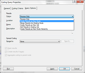
- The Query Options tab is where you will tell NVivo what you want to do with the Results of your query. The options will vary depending on the query type
- You can choose how you want the results to appear and where you want them to be saved
- You can add a description to the results (if they will be saved as a set or a node).
- Lastly, you can choose to Spread Coding and if so, to what units. (Reasons for and against will be discussed with the relevant queries below.)
- Note that hitting Run will both Run the query and save the query and results. Hitting OK will save the query as currently set up but not run it to get results. Cancel will simply close the window without saving anything
NOTE: There are limitless ways of performing these queries, depending on the items and the operators used. We can only show two examples. but given that the General and Query Results tabs are pretty much the same for each, the screenshots below are of the relevant Search Criteria tab only.
13.3. SCOPING THE QUERIES
Remember that all queries can be scoped to one or several selected files, a folder of files a Set of files or all sources (default). This can take place in the In bar of every query. Instead of agreeing to All Sources – use Selected items or Selected Folders

Figure 13.4
13.4. CODING QUERIES
Coding queries are probably the most frequently run query for most researchers. This query is very customizable and allows you infinite ways to examine how various codes have been used in your project. For this reason we only provide two sample queries – and several possible ways to vary outcomes.
CAUTION: none of the entire range of Coding queries work with Source Classifications and attributes – for this reason you hopefully used Node Classifications to get organised, i.e. using Node Classifications.
TIP: get into the habit of Adding to project (top left) to name and save the query – this saves the settings, i.e. the way you built the query – so that later you can re-run it or change the settings (but only temporarily) to experiment.
- In Explore ribbon tab – choose new Query/Coding query
There are two important tabs in the dialogue box – Simple and Advanced.
Simple means you can only ask for data coded by one node or by one attribute value – though you can add a second dimension by varying the scope (from All Sources, to Selected items or Selected folders).
Advanced means you can combine several different items in various ways (see below).
13.4.1 SIMPLE CODING QUERY
- Even if you are only going to do a Simple query – Add to project - In the example below a prefix has been used to name the query CQ-financially secure (later it helps to be able identify the broad category of the query you are reviewing, in the name itself)
- Having named the query – choose Coding Criteria tab

Figure 13.5
- EITHER at button for > Node / Select the node (thematic?) you want to examine (as shown in the example below OR at button for >Any node where (this is asking for Node Classification attribute value) – you can only choose one of these in a Simple Query
- You can add another dimension by scoping (or filtering) the query –see Figure 13.4
So…instead of running the query.
In …All Sources click on drop down arrow to either
- Select items (i.e.select particular documents, Sets, or Nodes (i.e. only in data coded by another node) Or… Select Folders i.e. folders containing sources
- Finally – in any query you can vary how you deal with the outcomes in the Query Options tab – these options vary depending on the type of query being performed – most of these options are self explanatory – but in case it is not clear – Create results as New Set – means that a Set of source files (shortcuts to actual documents) in which finds occurred satisfying the terms of the query, is created. Find the Set in the Collections function

Figure 13.6
13.4.2. ADVANCED CODING QUERY
In general, it is probably more common to use the Advanced tab since that allows more user flexibility. In this example (below), we have chosen to set up a query to determine what sections of source content have been coded to both the “Motivation” and the “Financially secure” nodes.
- Choose the Advanced tab – then Add to Project –in this example we are looking for the physical intersection or co-occurrence (AND) of two nodes


Figure 13.7
- Note also, that an AND has appeared at the Define more Criteria bar. Choose the node(s) in which you’re interested on the second bar
- Then hit Add to List button. AND means the togetherness or intersection of items in the data. If you accept this – and then select the second node (or any subsequent nodes-also on an AND basis) then the query will be performed finding only data where all the codes /nodes in this query, intersect
- Further versions of the same query could add attribute values (again on the AND basis) - and then additionally – vary the All Selected Nodes bar by clicking on the down arrow to choose Any Node where - Select Node Classification attributes and check the value of the attribute you want to add to the query criteria
- Get more complex by working incrementally - thus by employing different Boolean operators (see under the AND option) you can continue to narrow the focus of queries – or save relatively simple results at nodes and incrementally use the resultant nodes in further queries.
- OR..you can again be incremental by saving the results at a Node and building that node into new queries
- There are Boolean (AND, OR, NOT) operators and also Proximity operators
TIP: Experiment with queries you know the answer to in order to check that you are building queries correctly!
13.5. OVERVIEW OF MATRIX CODING QUERY
A matrix coding query is as if you were running multiple coding queries at once – usually you will be setting out to achieve one of several options:
- Comparing a selection of thematic nodes (or just one) across several attribute values
- Comparing a selection of thematic nodes (or just one) across e.g. Documents or Source Classification attributes
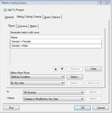
- Looking at how several nodes (or just one) co-occur (‘AND’), with other nodes. Other operators include ‘OR’ , ‘NOT’, ‘ PRECEDING’ ‘NEAR’ ‘SURROUNDING’ other nodes
The result will be a table where each cell represents the answer to a single query of the row and column – the initial view will be based on frequency – this can be varied – can be counting how many sources feature at all at a node, or number of coded passages (references), or number of words coded, or varied percentages etc. Each cell can be ‘opened’ to reveal relevant qualitative content. If the results of query is saved, you can return to the snapshot of the find over and over again. If you Save the ‘query’ i.e. Add to project you can re-run the query over and over again by double clicking on it.


Figure 13.8
- The results table of a matrix query will have Multiple cells. What type of frequency or shading shown in the cells - can be changed by right clicking in the table
- MOST IMPORTANT! Double clicking any one cell will open the results of that one e.g. co-occurrence, in the Detail pane. From there the qualitative data can be copied from any cell, meaning that this matrix query result can be used as a resource to come back to again and again when writing up
- EQUALLY IMPORTANT! Be sceptical about the numbers in the matrix – your qualitative sample is probably not designed to produce statistical significance. The numbers reflect personal interpretations and more importantly personal style of coding (big chunks coded or small chunks?) – it is the qualitative data behind each cell that s important – and that itself will be dependant on the thoroughness and consistency of your coding.
- Every matrix produces a rotatable 3D chart – view the chart from the side tables of the detail pane in which the result sits
13.6 Charting
This is all about standing back from the data while interrogating (see above after the results of a matrix coding query). A visual, but potentially quantitative look at who much coding has been applied in various places in your data. Charts can be created to show a variety of different things:
- See how coding in a source is broken down proportionately in that source
- See how coding is broken down proportionately across sources
- See how cases are broken down by attribute
- The results of a matrix query in 3D
- The quickest and easiest way to create a chart is to e.g. R-click on whatever it is in the List pane that you’re interested in charting> Visualize> Chart Document Coding . OR as below, right click on a code (here the code Wellbeing) Visualize> Chart coding for Node

Figure 13.8
- You can also generate a chart by going Explore Ribbon tab / Charts. This way will launch the Chart Wizard where you can choose what you’re seeing in a step-by-step fashion
Some additional thoughts on charts:
- Charts are very easy to use – but are limited
- Charts are useful - a good way of checking sample distribution or breakdown (an attribute by cases), for example
- Publishers will love them; researchers who think qualitative research is, at its heart, about numbers will love them
- Researchers who really need to integrate quantitative reporting with qualitative data will love them
BUT… charts are nearly always about a quantitative breakdown of your project in some way or another. Use them, profit (in terms of guidance and pointers) from them, but, as with all the quantitative breakdowns in software, be cautious and aware of what they are
13.7 Cluster Analysis
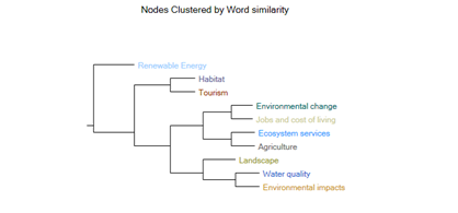
Cluster analyses allow a particular quantitative approach to the measurement and various visualisations of the relative associations of e.g. codes with other codes on the basis of word similarity or proximity.

Figure 13.9
Similar to charting – use Explore ribbon tab/Cluster Analysis to begin the process of building tree maps or cluster analyses – see the NVivo online Help? menu for more information on Cluster Analysis and Visualisation tools.

Figure 13.10
Here, nodes are clustered by their level of similarity of word usage . Or you can display sources similarly clustered by word usage similarity.
13.8 Concluding remarks
Since Charts and Queries are always produced at a point in time, remember that there is a purpose in saving snapshots of the results – but also
With queries, the results are snapshots if you save them under Query Options.
The Query itself is dynamic (if you use Add to Project button) since you can re-run it
With Charts they are correct at a point in time – you can export them (as a graphic) in order to be able to track back or retain information at different stages of work at this level.
Ann Lewins, Christina Silver and Jen Patashnick 2014
