Using Software in Qualitative Research
A Step-by-Step Guide
Chapter 8 – Retrieval (TRANSANA)
Download the pdf for this chapter guide here.
Chapter 8 in the book focuses on retrieval – a crucial aspect of qualitatively coding data. Yet there are many aspects of this which lead to other things. While looking at one batch of coded data you may want to delve deeper and recode it. There is an aspect of interrogation, using filters to examine particular catchments or subsets of data, cutting data in different ways – vertically in one document or horizontally across all. See all coloured illustrations (from the book) of software tasks and functions, numbered in chapter order.
Continuity
Horizontal and Vertical cuts
Filtering devices
Recoding
Generating reports
Quantitative outputs
Basic Retrieval of Coded Data with Transana by David K. Woods, Ph.D., Transana’s Lead Developer and Joseph H. Woods, Intern
One of the analytic advantages of using Collections is that relevant Clips and Snapshots are already gathered together in one place when it’s time to examine them. When you’re using Keywords to signify analytic categorization, you need to perform a Search to gather the appropriate Clips and Snapshots together for you before you can begin to explore the data.
Let’s look at what we have coded with the Keyword “Gendered Techniques : Objectification” in chapter 7 exercises, section 7B. This code was applied to clips across a number of Collections. Since we want to look for only a single code, Transana’s Quick Search is perfect. We can initiate a Quick Search by right-clicking the desired keyword in the Database window and selecting “Quick Search” from the menu.

This gives the following results, which appear in the Database Tree’s Search node:

You can see that Transana returns Clips and Snapshots, arranged in Collections, as the result of the Quick Search request. The Search Results node acts just like a regular Collection. But Search Results are not permanent in Transana. You can double-click Clips and Snapshots to load them in Transana’s main interface. You can right-click objects in a Search Result to request Reports and Play All Clips. You can use “Locate Clip in Episode” and “Show Snapshot Context”.
You can rename and re-organize items and drop false positive results using “Drop from Search Result” from several of the right-click menus. None of this will affect the original data that was searched to create this Search Result. (Please note, however, that if you load a Clip or Snapshot from a Search Result, changes in coding WILL affect the originating data object. It is work on the Search Results node in the database tree that is not permanent.) The notion is that you sometimes need to manipulate data a bit to figure out whether a given search has produced meaningful results, but that you don’t want to harm your data by doing so.
If you do discover something important within a search result, one option you have is to embody that discovery in a Collection by converting the (manipulated) Search Result node into a permanent Collection. You can accomplish this by right-clicking the main node for a given Search Result, called “Gendered Techniques : Objectification” in this example, and select “Convert to Collection” from the popup menu. When you do this, copies of all of the analytic artifacts displayed in the Search Result are made and added to the project database.
There are a number of ways to examine information about the coding you have done with your data. First, let’s look at the information available about Clips and Snapshots in Collections, data gathered together by analytic meaning regardless of source media file. Lewins and Silver refer to this as “Horizontal Retrieval” of data.
To generate a text-and-image-based report with general information about all of the Clips and Snapshots gathered together in a given Collection, right-click the Collection and select the “Collection Report” menu item. If you want this report for all Clips and Snapshots in all Collections, you can initiate this report from the main Collections root node in the database tree (although generating this report on a large database can be time-consuming.) You can also generate the “Search Collection Report” by generating the report based on a Collection in a Search Results Node.

Transana will generate a report with a variety of details about all Clips and Snapshots in the selected scope, the Collection used to initiate the report. The image above shows a single Clip record and a partial Snapshot record from a report made up of the 40 Clip records and 5 Snapshot records used to analyze the Gardener ad.
Is appropriately configured, the Collection Report includes a very basic Summary section at the end of the report.

The report’s Filter Dialog allows significant customization of the report. You can select what data elements to include in the report, as well as what Clip, Snapshot, and Keyword information to include.
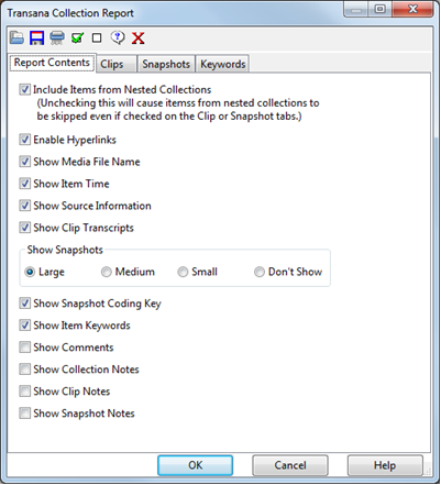
The Filter Dialog allows you to save your filter configurations. This allows you to create a custom view of your data, which can easily be loaded and used on your data in the future. This allows you to easily repeat the embodied analytic view as your analysis proceeds and your data changes.
If so configured, each Clip and Snapshot record in the report includes a hyperlink, which will load the data object requested into Transana’s main interface for further exploration, allowing you to stay extremely close to your source data. The report can be edited by hand if needed, and can be exported as a Rich Text Format document that can be loaded into a Word Processor. (Clip and Snapshot hyperlinks are not exported, as they require Transana’s infrastructure to function correctly.)
A graphical report called the Collection Keyword Map shows the patterns of coding in all clips within a given Collection. Please note that the horizontal axis of this report is an artificial time line created as if all clips were placed end to end and is not interpretable.

This example, from the Gardener ad, allows us to see the dominance by the Keyword “Gendered Techniques: The Gaze – Female” in our “Shots of Women” Collection and to see that close-up shots are often associated with Objectification and Sexualization in this commercial. Clicking a bar in this report loads the underlying Clip or Snapshot object into Transana’s main interface, allowing easy exploration of report elements in the source data. This report can be exported to JPG format for inclusion in analytic write-ups, articles, and reports using the “Save as JPG” button in the report’s toolbar.
Saving a report to a JPG image allows you to save a snapshot of your data analysis at a particular point in time during your analytic process. The image is exactly the same every time you view it. In contrast, saving a Filter Configuration allows you to create an analytic view or lens on your data set. When you load that Filter Configuration at a later time, the report will reflect changes you have made in your data. Both of these can be useful in the analytic process.
Now let’s look at the information available about Clips and Snapshots taken from or associated with Episode, data derived from the same source media file regardless of how it is used analytically within Transana’s Collection structure. Lewins and Silver refer to this as “Vertical Retrieval” of data.
To generate a text-and-image-based report with general information about all of the Clips and Snapshots taken from or associated with a particular Episode record, right-click the Episode and select the “Episode Report” menu item.
This report is almost identical in form to the Collection Report described above. It selects and gathers data completely differently, but displays it in an identical format with very similar options and functionality, including the Summary section and in the Filter Dialog.
There are a number of graphical reports available based on source media file. Similar to the Collection Keyword Map described above, you can right-click the Episode you would like to examine and click the ‘Keyword Map’ menu item. This creates a report where the horizontal axis represents the time line of the source media file showing coding applied to the file across time. Unlike the Collection Keyword Map, this time line is meaningful and interpretable. Clicking any of the bars representing Keywords will load the corresponding Clip in Transana’s main interface. The Filter Dialog controls many aspects of the appearance of the Map, and you can export the image to a graphics file by pressing the “Save to JPG” button in the upper left-hand corner of the Keyword Map window.
You may notice that the Keyword Map is very similar to the Keyword Visualization. If you want to print or save a Keyword Visualization, use the Keyword Map instead.
If you right-click a Series record, you will see a number of report options designed to present information from multiple related source files that have been placed in the same Series.
The Series Keyword Sequence Map presents an identically-formatted Keyword Map for each Episode in a Series, all in a single report. We can use the Filter Dialog to pare it down to just the Episodes we would like to analyze. If we save our filter configuration using the name ‘Default’, this filter will automatically be applied when the report is created again. (Deleting the default filter configuration can restore it to its original state.)
We wanted to represent some of the differences between our ‘Gardener’ commercial and its precursor, a 1994 advertisement named ‘Diet Coke Break,’ of which ‘Gardener’ is a spiritual sequel. We transcribed and coded the two videos, and used the Series Keyword Sequence Map to represent them side-by-side.

The configuration itself was easy to build. Simply uncheck all Episodes but the two we are using, or use Transana’s Uncheck All feature and recheck the two you need manually.
The same goes for our Keywords, which can also be recolored on this screen by selecting a Keyword and assigning it a new color below.

There are many interesting things to notice in this graphical report. For just one example, take a look at the coding of “Gendered Techniques : The Gaze – Female” and “Gendered Techniques : The Gaze – Male” in the two media files. In 1994, the male gaze was not present, as the man in the commercial did not know he was being watched, while in 2013, we see an interplay of the male and female gaze as the characters in the ad look at each other and interact. This difference is ripe for theoretical interpretation, to say the least.
But suppose that, instead of wanting to see how our coding plays out over time, we would rather get either concrete or percentage-based representations of the amount of time a Keyword is present. This can be achieved by the other two Series Keyword visualizations, namely the Series Keyword Bar Graph and Series Keyword Percentage Graph.
The Series Keyword Bar Graph displays cumulative seconds of coded time, aggregated for each keyword. We used the Filter Dialog to examine only these two ads and their Keywords.

This view is a very useful one for comparative examination. For example, in the 60-second ‘Gardener’ commercial, we can see that Coca-Cola is on screen for 10.7 seconds. Simply hover your mouse over the bar corresponding to the code “Shot Types: Product Present” to show the amount of time coded for that Keyword.

The ‘Diet Coke Break’ advertisement, however, features 18.1 seconds of Coke – either symbolically or literally – over its 45 second runtime. This difference is worth some additional consideration and theoretical interpretation.

The Bar Graph only gives us aggregate seconds of coding, however. In addition, any overlapping Clips recoded with the same Keyword will influence the time presented in this Graph. If we wish to see relative proportions of Keyword coding, we can instead use the Series Keyword Percentage Graph.

For example, with some careful reduction of our Filter to include only mutually-exclusive codes, in the following image we can see the relative proportions of each commercial in which women are on screen – and see a difference not apparent from the relatively equal-looking bars on the Bar Graph.

We see less time (as a percentage of the entire ad) spent showing the women in the 2013 ad compared to the 1994 ad. The percentage of time spent on men stays the same, and the difference appears to be made up of shots that are not of people at all, something we didn’t see at all in 1994. Looking at the shots coded as not being of people might help us figure out how to interpret this shift over time.
The Percentage Graph has some downsides, though. In order to use it, we must understand that its percentages represent percentage of total coded time presented in the graph, not percent of the length of the media file. This means that any Clips with multiple codes or any overlapping Clips will skew the percentages and make them less meaningful. In order to prevent this, ensure that your filters are configured very carefully.
At any stage in your work it will be necessary to cycle between the creation of clips, coding and writing to keep track of subtle insights and progress see Chapter 10 exercises next
David K. Woods 2014