Using Software in Qualitative Research
A Step-by-Step Guide
Student Resources
Chapters 10,11 & 13 - Mapping, Managing Interpretations and Interrogation
Download the pdf for these chapter guides here.
ATLAS.ti and Chapter 13 – Interrogation
Chapter 13 in the book discusses interrogation of data that can happen at varied levels and at many moments during analysis. Already in Chapter 6 we referred to Text search tools where the content is explored. Chapter 5 discusses basic retrieval and the ways this can be varied. Further interrogation can also happen in terms of coding work you have previously achieved. You might wish to discover relationships between codes which co-occur in some way in the data or need to compare them across subsets of data (indicated by the application of variables or attributes to data). Types of queries vary from simple to complicated tasks; summarized, charted information where the results are already available in the background is available in some software. See all coloured illustrations (from the book) of software tasks and functions, numbered in chapter order.
Sections included in the chapter:
Incremental and iterative nature of queries
Creating signposts for further queries
Identify patterns and relationships
Qualitative cross tabulations
Quality control, improving interpretive process
Tables and matrices
Charts and graphs
Some of these themes are picked up below.
Data Analysis
If you click on the ATLAS.ti Analysis menu, you see a number of analysis options. In the following you find exercises for the Codes-Primary Documents Table, the Code Cooccurence Tool and the Query Tool.
In order to prepare the project for these exercises, I used the Word Cruncher (first option in the analysis menu – see also the Chapter 6 exercises) to check which are frequently occurring words in the newspaper articles that are part of project B. Based on the frequently occurring words that I reviewed in a Word Cloud (Figure 1), I coded the data using the auto coding function. I did not further investigate the data segments that were coded, so please don’t take the project as a good example for a coded project! It is a “quick & dirty” project, but it serves well (hopefully) to help you understand the analysis tools.
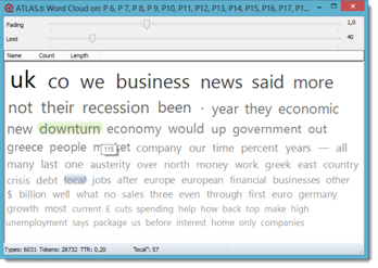
Figure 1: Word count for documents presented in form of a word cloud
- To go through the following exercises, download the copy bundle file of this project from the companion website (case study B_analysis exercises 1 to 4) and unbundle it
NOTE: You find a detailed instruction on how to unbundle copy bundle files at the end of this chapter.
Codes-Primary Documents (PD) Table
The Code-Primary Documents Table is a useful tool, if you want to compare and contrast on the document or case level. It allows you to compare the distribution of codes across documents or document families, depending on how your cases are defined. The initial output of the analysis is quantitative in form of an Excel table. Usually an analysis with the Codes-PD Table is followed up by a more specified query in the query tool.
Let’s take a closer look at the sample project first:
- The project contains 69 documents (P6 to P74), thus the focus group data are excluded. If you open the P-Docs Manager, you see that the documents are sorted into various document families grouped by local and international media and by years 2008 to 2012
- Open the Code Manager to take a look at the codes. You find one code family containing all the country code, i.e. the countries that are written about in the articles, and the content codes used for auto coding the material like bank, business, community, company, council, credit or dept. Those codes have been grouped into code families in order to be able to access keywords that relate to a similar topic like communal issues, economy, finances, politics and work
Exercise 1
For this exercise, I want you to examine the following research question: Is there a shift in the various issues that are discussed over time (2008 – 2012), or between local and international media?
Obtaining quotation frequencies per code and document (group)
- To find an answer to this question, select Analysis / Codes-Primary Documents Table
- Select all Code Families and click on the button with the right arrows to move them into the field Selected Codes / Families:
- Select the PD families for the years 2008, 2009, 2011, 2012 (actually, these are Super-PD families. You can see this at the red color)
- Look through the standard setting on the right hand side of the window. If you want different settings than the standard options, make some changes. Then click Create Report
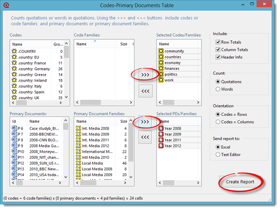
Figure 2: Codes-Primary Document Table
- Excel opens and you need to confirm that Excel can convert the table. The outcome looks like this. I highlighted what might be interesting issues and differences to look at
|
|
Year 2008 |
Year 2009 |
Year 2011 |
Year 2012 |
TOTALS: |
|
Communal issues |
4 |
40 |
11 |
5 |
145 |
|
countries |
8 |
7 |
45 |
41 |
101 |
|
economy |
127 |
167 |
132 |
150 |
576 |
|
finances |
51 |
71 |
70 |
79 |
271 |
|
politics |
11 |
6 |
40 |
49 |
106 |
|
work |
46 |
93 |
52 |
93 |
284 |
|
TOTALS: |
257 |
407 |
373 |
446 |
1483 |
Interpreting frequencies always needs to be done with care. Take a look at the totals: the number of quotations (coded segments) for each year is not the same. Hence, for a quantitative comparison you would need to calculate relative frequencies for each cell.
What we can see is that issues around economy and finances occur in about the same frequency across each of the four years. Communal issues seemed to have been more important in 2009.
- Practice the tool again and check whether communal issues are discussed more in local than in international papers.
Answer: …?
- Ok, now we know that communal issues were only written about in the local media. As the code family communal issues groups together four codes, we can ask as follow up question: What type of issues are these?
- The keywords included in the code family communal issues are: community, council, county and pubs. Create a new Codes-PD Table including these four codes and the PD family ‘Local Media 2009’. Before you add these new items, remove the code and PD-families that are currently listed in the selected objects fields first. The results of the two last queries are shown in Figure 3
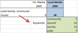
Figure 3: Issues around community in the local media in 2009
Query tool
Exercise 2
For this exercise, let’s take a look at the qualitative data behind the numbers in the table shown in Figure 3 above. For this, we need to make use of the Query Tool in combination with the Scope button. Let’s take a look at the 2009 data segments that include the word ‘pubs’.
Combining a simple code query with a variable
- Open the Query Tool: Analysis / Query Tool
- Double-click the code ‘pubs’. In the result pane at the bottom right, you see a list of 9 quotations. These are all quotations found in the data set
- To reduce the findings to the 2009 local date, click on the Scope button that you find at the bottom right of the query tool. This opens the Scope of Query Window. Position it next to the Query Tool. At the top left, you see the list of PD-families. Select the family ‘Local Media 2009’
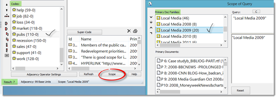
Figure 4: Combining a code query with a variable (PD Family) via Scope
- ·As result we get the 7 quotations. Take a look at the result pane in the Query Tool window. The scope of query window only serves as tool to set filters. We already knew that we will find 7 quotations from the Codes-PD Table. To look at the content behind the number, click each quotation in the result pane. The respective document will be loaded and the quotation will be highlighted in context
- If you want to output all 7 quotations, click on the printer icon on the top left of the result pane and select the output option ‘full content’ or ‘full content, no meta’. The latter option provides a shorter output only including the data segment plus one line of reference
- Read through the quotation and summarize the findings in a memo (see Exercise 6)
Exercise 3
Did you notice that the numbers in Figure 3 do not quite add up? ATLAS.ti found 40 quotations coded with the keywords around community. Exporting the values for each single code, we end up with a total of 48. The reason for this is that some of the segments are coded with two or more of the communal issue codes. We can find the overlapping quotations by using the cooccurence operator in the query tool.
You may already guess that it might be the two words county and council, as in the UK county council is the elected administrative body governing an area known as a county.
Using proximity operators in the query tool
- To prepare the query tool window for a new query, press C in the scope of query window to reset the scope
- Likewise, press C in the query tool window to clear the code in the query tool.
- Double-click the code ‘county’
- Double-click the code ‘council’
- Click on the COOCCUR operator (last one in the list of operators, Figure 4). ATLAS.ti finds 4 quotations were council and county occurs within the same coded segment
Creating a Super-code
- If you want to retrieve these data segments later on once again because you are interested in the role of UK county councils, you can preserve this query by clicking on the Super-Code button. Accept the suggested default name or enter a new one
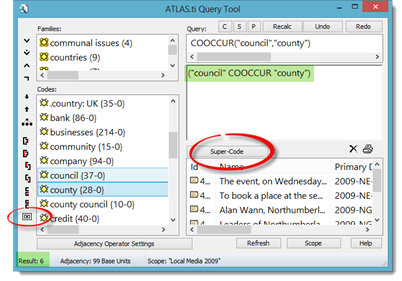
Figure 5: Query for exercise 3
Code Cooccurence Table plus follow-up
The code co-occurrence tool finds segments where two codes overlap. There are five possibilities of overlapping: A coded segment can be nested within another one, it can be enclosed by another one, it can be overlapped, it can overlap another segment, or one segment is coded by two codes. The Code Cooccurrence Tool queries all of these five possibilities.
Exercise 4
In addition to the content codes, the data has also been coded with country names. Therefore an interesting question is which of the issues are mentioned in relation to what country?
Cross-tabulation of codes
- Open the Code Cooccurence Table from the Analysis menu
- Take a look at the toolbar. Towards the right, you see a button with a C. If activated, ATLAS.ti calculates a C-coefficient. Deactivate this option as we only want to look at quotation frequencies. We need different data source material for this option to make sense. For more information on the C-coefficient take a look at the manual or at the book written by Friese (2014): ‘Qualitative Data Analysis with ATLAS.ti’
- On the right hand side of the window you see the codes that you can enter for the columns and rows. Under Columns, select all country codes and click on the Add button. Under Rows, select all content codes and click on the Add button. The table now wills with numbers

Figure 6: Displaying data based on code co-occurrence results
- If you click on a cell, a drop-down list opens showing the quotations. Position the table so that you can see the data as well. Then click on a quotation in the drop-down list. It will be shown in context
Cross-tabulation of codes by document groups
- Filter settings can be applied to the table as well. But before we try that, let’s take out the codes that are not applicable: community, council and county. Remove them from the rows. They just add clutter to the table
- Now, let’s check whether there is a difference between local and international media: From the main menu, select Documents / Filter / Families and select ‘International Media’. You see that ATLAS.ti recalculates the table. There is little change in numbers. Now, set the filter to ‘local media’. What do you observe?
- Do the same for years. And voila, what do you see? A lot is happening in the year 2012 and especially in the column ‘Greece’
- If you want a quantitative output, click on the Excel button in the toolbar. As output destination select File & Run
If you want qualitative output, we currently still have to use the Code Cooccurence Tool in combination with the Query Tool. This will change at some point, probably still as new feature of version 7. You will then be able to create a report directly in the Code Cooccurence Tool.
Once again, a proximity query in the query tool
- Take a look at the column for the country ‘Greece’. What type of issue are you interested in? Let’s take for instance a look at the keyword ‘economy’
- Open the query tool
- Double-click the code ‘economy’
- Double-click the code ‘country: Greece’
- Click the COOCCUR operator
("economy" COOCCUR ".country: Greece")
Note: It does matter in which order you enter codes when using any of the proximity operators. ATLAS.ti cannot export just the overlapping part; it always outputs the quotations for the first code that you entered. Here: economy. If you wanted to focus on Greece and what is written about it in the context of the word economy, you would add the query the other way around (country:Greece COOCCUR economy).
- ·Click on the Scope button and filter the results by year. You can use the international media PD-families, as there will be no results for local media
Further analysis of the Focus Group Data
As you need to code respondent characteristics in focus group data (or any other data where your documents are not the cases), the Code Cooccurence Tool in combination with the query tool are the tools you need to use for further analysis. Let’s take a look at the coded focus group data. For the following exercises, download the copy bundle file ‘case study B_ analysis exercises 5 to 7’ from the companion website.
Exercise 5
After you have installed the file, open the Code Manager to take a look at the codes. All sociodemographic codes begin with a hash sign (#). After that you see the list of content codes. Let’s take a look which effects might be the stressors that make people worry and that cause distress.
Cross tabulating codes
- Open the Code Cooccurence Table
- Select the emotion codes and enter them into the columns
- Select the codes starting with ‘effects…’ into the rows. Do you find something interesting?
Let’s focus on the two codes ‘emotion: being worried’ and ‘emotion: distress’. Thus, remove the other two from the columns. Also remove those codes from the rows that do not apply (n/a).
- Now, add the socio-demographic codes for gender and employment status to the rows. This is what we get:
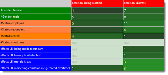
Figure 7: Exploring possible causes for emotional stress
Feeling distressed appears to affect more those that are employed in comparison to other groups. An explanation for the higher distress of those that are employed could be that they feel that the moral at work is bad and that job conditions have been getting worse. Based on these initial findings, we can explore what might be other stressors.
Let’s check whether the location (rural, urban) has an effect as well. As the focus group participants were not mixed on the basis of location, i.e there are two focus groups made up of participants from rural areas and 3 from urban areas, we can use PD Families as filters.
- Open the P-Doc Manager and position it either next to the code cooccurence tool or underneath the table (see Figure 8)
- Right-click on the PD family ‘rural) and set it as global filter. Observe what is happening in the code-cooccurence table
- Next set the global filter for the PD family ‘urban’
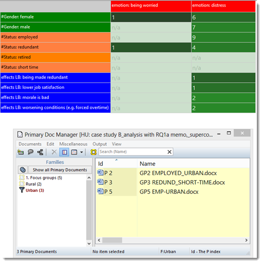
Figure 8: Checking whether location (rural, urban) has an effect of emotional distress
The resulting tables tell us that feelings of distress have been voiced much more by respondents from urban areas, and worries by respondents from rural areas. Let’s keep the latter finding in mind as we should explore it a bit further as well. For now I would like to continue the analysis on the issue of distress.
- Take a look at the code group ‘finance’ and cross tabulate it with the employment status. Thus, we create a new 2 x 5 table (status as column codes, finance as row codes). If you take a look at the numbers, you have to take into account that the number of responses in each group is not the same. We have many more speaker sections of employed respondents (84, as compared to 23 redundant, 40 retired and 9 short-time). Nonetheless, financial issues do seem to be of more concern to the employed

Figure 9: Cross-tabulating employment status with financial issues
Creating super codes in the query tool and using the super codes for further analysis
Mmh, you may wonder. Who is more distressed by it, males or female? In order to examine this, we need two super codes: one for employed males and one for employed females.
- Close the Code-Cooccurence Table
- Open the query tool
- Double-click on the code #Status employed. Double-click on code #Gender:female
- Select the AND operator. Click on the Super-Code button. Accept the default name or enter a new one
- Repeat the process for the two codes #Status employed and #Gender:male
- Close the query tool
- Create a new Code-Coocurrence Table, entering the two new super codes into the columns and the finance codes into the rows. Then add the two emotion codes ‘distress’ and being worried’ (Figure 10)
- What does the table tell you?

Figure 10: Cross-tabulating status & gender with the codes from the categories ‘finance’ and ‘emotion’
Above we have seen that ‘feeling distressed’ has been mentioned equally by both male and females. What could be other stressors for females if not the finances? Compare males and females and their status. You will find that in the sample data we have only females that have been made redundant and that this relates to feeling distressed.
Have you noticed in Figure 7 that being worried has been mentioned quite often from respondents from rural areas? What could be the reasons for that? Explore the cooccurence of the issues mentioned with the code ‘emotion: being worried’. You find the answer in the network view shown in Exercise 7, Figure 13.
After getting an overview of what is going on, it is now time to actually take a look at the data behind the numbers. By now, you should know which tool you need for this I.E. the query tool. It is also time to write down what you found so far. For this, we will create a ‘research question memo’ in the next exercise.
ATLAS.ti and Chapter 10 – Managing Interpretations
Chapter 10 n the book is all about managing interpretations; managing where and how you make analytic notes, using software structures to ensure your thoughts do not get forgotten or your notes lost. Ways of expressing or visualizing connections and relationships are sometimes provided in software and help in the generation and management of the ideas that you have about the data. The literature that informs your work is very important and these software programs can be used in many different ways to manage cross referencing with substantive data or to manage the literature review itself. See all coloured illustrations (from the book) of software tasks and functions, numbered in chapter order.
Sections included in the chapter:
Writing as continuous analysis
Critical Appraisals of literature
Analytic memos
Process memos
Definitions
Linking notes to data
Integrating notes with other work
Visualising memos
Taking Notes in ATLAS.TI – Writing Research Question Memos
We started the process of creating memos soon after creating a project. There is much more to say about them:
Research question memos are analytic memos. I describe them as places where you develop the interpretation of your data step by step. At the beginning of analysis, your research question memos may simply contain descriptions and summaries of your data. If you take the analysis a step further, some of the descriptive memos may serve as building blocks for more abstract and theoretically rich memos (see also Bazeley and Richards, 2000: part 6, Corbin and Strauss, 2008:119).
In qualitative research, we generally do not start with hypotheses but in most cases we have some research questions. When using an inductive approach, researchers develop questions and hypotheses along the way. If you begin your project with some research questions in mind, you can create research question memos very early on in the analytic process, adjust and modify them, and add some more with progressive analysis.
Exercise 6
A fully developed research question memo:
- has a proper title that tells you what it is all about;
- can be identified as an analytic memo by its type;
- begins with a well-written research question, possibly followed by sub questions;
- includes the query (!);
- contains an answer to the query – when you work on a memo over a prolonged period of time, you can also insert the date and time to mark your progress;
- contains your answer and interpretation;
- is linked to quotations that illustrate the points you are making and supports your analytical claims.
Creating and writing a research question memo
- Open the Memo Manager and create a new memo.
- Enter the title ‘RQ1a: Causes of emotional stress’. For the purpose of linking memos to data segments, it is a good idea to keep the title short as the memo title will show up in the margin area.
Note: Research question 1: ‘Implications of financial downturn’ is too general in order to answer it all in one memo. We need to break it down into smaller sections and therefore I entitled the memo RQ (for research question) 1a.
- Change the memo type to ‘Analysis’
- Type the full research question into the memo editor: ‘What are potential causes for emotional stress like being worried a lot and feeling distressed and how is this related to socio-demographic characteristics like gender, location and employment status’
- Next write down how you did go about finding an answer to this question (see step-by-step instructions in exercise 5)
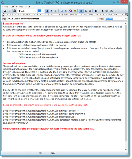
Figure 11: Example of a research question memo
Taking a look behind numbers and linking memos to data
At the end of exercise 5, you were asked to take a look behind the numbers produced by the cross-tabs by using the query tool. Here are some example queries that add more meaning to the numbers:
("*#Status: employed & #Gender: (fe)male" COOCCUR "emotion: distress")
("*#Status: employed & #Gender: (fe)male" COOCCUR "emotion: being worried")
("*#Status: employed & #Gender: (fe)male" COOCCUR "financial issues")
("*#Status: employed & #Gender: (fe)male" COOCCUR ("effects LB: morale is bad" | "effects LB: worsening conditions (e.g. forced overtime)"))
While reading the data, you probably come across some interesting quotes that you want to cite later on in your report. For instance, it is noticeable that even though both men and women are distressed, women are much more emotional about it than men. So you may want to pick two example quotes, one from a male and one from a female respondent. This is how it works:
- Save the memo content
- Minimize the memo editor. Highlight one quotation from a female respondent related to distress. Then drag and drop the memo from the Memo Manager across the windows splitter to the left side of the HU editor. The memo icon and title shows up in the margin area (Figure 12)
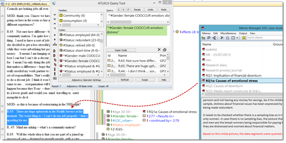
Figure 12: Linking a memo to a quotation
- Repeat the process and link the memo to a good quotation from a male respondent
- Take a look at the Memo Manager. The count for groundedness has gone up. Double click on the memo entry. As in the Code Manager, a window pops up showing you all quotations linked to this memo. When you click on the quotations, they are highlighted in context and you can see where the memo is attached
Creating output
That, however, is not the end of the story. What we want to do next is to output the memo, including the quotations. When you set up your research question memos as described, the output can be used as a building block for your research report.
- Select your RQ1a memo and then the option Output/Selected Memo with Quotations
- Choose Editor as the output destination
The memo output includes everything you need to write the results chapter of your research report or paper (see below). It also adds transparency to your analysis. If someone asks how you derived your results, you can show your research question memos. It just takes a minute or two to spell out the query, and the return for this effort is manifold. It adds a lot to your analysis in terms of trustworthiness, credibility, transparency and dependability – in other words, the quality criteria by which good qualitative research is recognized (see, e.g., Seale, 1999).
MEMO: RQ1a: Causes of emotional stress (2 Quotations) (Team, 2014-01-12 19:57:51)
P 2: GP2 EMPLOYED_URBAN.docx:
(30:30), (43:43)
No codes
No memos
Type: Analysis
Research question:
What are potential causes …..
In order to find an answer to this question, the following analyses were run:
- Cross-tabulation of emotion codes by gender ………
Summary description:
The results of the cross-tabulations show that the focus-group respondents that were sampled express distress and worries as implication ………
Based on this initial picture, the data segments were queried using the query tool:
("*#Status: employed & #Gender: (fe)male" COOCCUR "emotion: distress")
("*#Status: employed & #Gender: (fe)male" COOCCUR "emotion: being worried")
("*#Status: employed & #Gender: (fe)male" COOCCUR "financial issues")
("*#Status: employed & #Gender: (fe)male" COOCCUR ("effects LB: morale is bad" | "effects LB: worsening conditions (e.g. forced overtime)"))
Continue summarizing and interpreting what you learn from reading the data segments….
………………………………………………………………………………………………………………………………………………………………………………………………………………………………………………………………………………………………………………………………………………………………………………………………………………………………………………………………………………………………………………………………………………………………………………………………………………………………………………………………………………………………………………………………………………………………………………………
Good Quotes
P 2: GP2 EMPLOYED_URBAN.docx - 2:66 [R.10: Blimey that’s not happen..] (30:30) (Super)
Codes: [#Gender: male - Family: sociodemographics] [#LOC_urban - Family: sociodemographics] [#Status: employed - Family: sociodemographics] [Z-R.10 - Families (3): Z-EMP-EMPLOYED, Z-MALE, Z-URBAN]
Memos: [RQ1a: Causes of emotional stress]
R.10: Blimey that’s not happening at my place. We don’t have a union – too small a place but you know - its not small enough to be personal. So they – the bosses I mean er well you don’t get the feeling it matters much to them. We’ve got an overtime ban – that means we work overtime but we don’t get paid for it because they say they are under pressure and jobs are at risk blah blah. Its causing a lot of stress – people off sick and stuff.
P 2: GP2 EMPLOYED_URBAN.docx - 2:57 [R.65: There are huge upheavals..] (43:43) (Super)
Codes: [#Age 30-39 - Family: sociodemographics] [#Gender: female - Family: sociodemographics] [#LOC_urban - Family: sociodemographics] [#Status: employed - Family: sociodemographics] [Z-R.65- - Families (4): Z-AGE-30-39, Z-EMP-EMPLOYED, Z-FEMALE, Z-URBAN]
Memos: [RQ1a: Causes of emotional stress]
R.65: There are huge upheavals in the Health Service at the moment. The worst thing is – I can’t do my job properly – that’s upsetting for me.
Quoting data segments in reports
In order to reference a quote from an ATLAS.ti project, my suggestion is to use the quotation ID plus the location in the document. For instance:
‘R.65: There are huge upheavals in the Health Service at the moment. The worst thing is – I can’t do my job properly – that’s upsetting for me.’ (2:57, 43:43)
Alternatively, you can use as reference (P2, 43:43) = document number, start and end position of the quotation.
You need to explain the references once, for example in a footnote. The coded documents where the quotation can be found in the data can be included as digital attachment to a report, thesis or dissertation. A Web-based publication such as an html document is also possible. Most choose the PDF output of the coded documents. This is available for text, image and PDF files.
To create a PDF output of your coded documents:
- Select Documents / Output / Print with Margin.
As soon as you select the print with margin option, the screen view changes so you can see what the output looks like on paper or in a PDF file. Everything on the page is within the white area; everything off the page is shown in the grey area. You may need to adjust some settings to fit everything on the page and to create the output you want:
- If some codes fall off the page on the right hand side, I suggest that you set the page layout to landscape: Project / Printer Setup
- You can also adjust the windows splitter (move it to the right or left) and change the font for the codes (right click in the margin, select the option Set Font) to create the view you want
- If you want to create a PDF file, a PDF writer needs to be installed on your computer. Nowadays you can find free versions online. When creating the output, the printer dialogue opens. Choose the PDF writer as your printer. Then the document will not actually be printed but saved as a PDF file. If you select a segment of text, only the selection will be included in the printout
Managing interpretations through writing and other aspects discussed above is enriched by the ability to express ideas and their connections in a visual way using the network tool. See the next Chapter 11 exercises below
ATLAS.ti and Chapter 11 – Mapping
Chapter 11 discusses some of the varying principles, functions and rationales behind mapping tools where they are available in software. Mapping in a graphic sense may relate to theoretical models or simply be a way of stepping back from the data to express, visualize and communicate connections that are beginning to be observed. See all coloured illustrations (from the book) of software tasks and functions, numbered in chapter order.
Sections included in the chapter:
Traditions of mapping
Specific functions and specialities
Mapping to express theory
Visualizing links between text passages
Visualizing co-occurring codes
Linking concepts
Layers, creating, hiding and revealing them
Creating Network Views
Last but not least you can visualize your findings in a network view. The story told above could for example be illustrated like this:
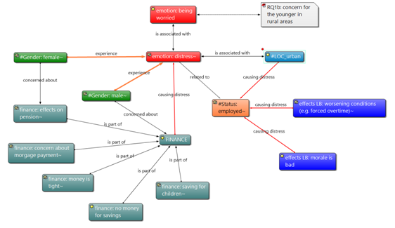
Figure 13: Network view illustrating the findings of Exercise 5
Exercise 7
Learning how to link
- Open the Code Manager and choose the following codes by holding down the CTRL key:
- emotion: distress
- emotion: being worried
- #Loc_urban (does not exist, you need to create it)*
- # Gender: female
- #Gender: male
* It is common when working with network views to create new codes in order to express the kind of relation you found in the data.
- Then click on the network symbol in the toolbar of the manager·
 A network view editor will open. As a title, the name of the selected code(s) is chosen. The window contains the code you have selected. If you want to add more codes later, move the network view window next to the Code Manager and drag and drop other codes into the network view
- Select the code node ‘emotion: distress’ with a left mouse click. A red dot will be displayed in the top left corner of the node. Drag the red dot with your mouse to the code node ‘emotion: being worried’ and release the mouse button. A list of relations will open
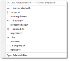
Figure 14: List of code relations
 Depending on the type of project you are working with, the list of relations on your computer screen might be shorter than the one shown in Figure 14. In addition to the default relations that ATLAS.ti provides, it includes a few others that I have created for the sample project. Further below I show you how to create new relations.
- For now, select the ‘is associated with’ relation. This relation is a symmetric relation showing a double-ended arrow. It indicates that the two codes are related somehow but no direction can be specified
Let’s try out another way of linking:
- Left click on the code note ‘emotion:distress’ again so that you see the red dot. This time click on the Link Nodes button in the toolbar. Drag the black line on top of the code node ‘#LOC_urban.’ Choose the ‘is associated with’ relation again
- Next, link one of the gender code nodes to ‘emotion:distress’. This time select the option Open Relation Editor as I want to show you how to create a new relation. In Figure 13, I have linked these two nodes with a directed (transitive) relation that I named “experience”
- In the Relations Editor, select the menu option Edit / New Relation. This opens the relation editor (Figure 14). All input fields are empty and can now be filled with new information. If you don’t see the Edit menu, make the editor window a bit larger
- Enter an internal ID (e.g. EXP)
- Enter label 1, label 2 and the menu text (see below)
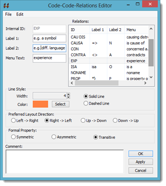
Figure 15: Creating a new relation in the relation editor
- Then, select the width and color for the line
- Set the formal property to Transitive (directed, one arrow pointing in one direction e.g. to express causal linkages)
- Click on Apply to accept the new entries. Click OK
Exploring the links
- The link labels are interactive. Right click on a link label and explore the options like flipping a link, changing the relation or cutting a link
- Each link can be commented individually. Try it. All commented links are marked with a tilde (~) as you already know from other commented objects in ATLAS.ti
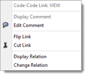
Figure 16: context menu for relations
Importing nodes into an existing network view
You can import objects into a network view editor via drag and drop from all managers or the margin area. Another option is via the menu Nodes / Import Nodes. Try it out:
- Import the codes of the finance category (main category code plus all sub codes)
- The imported nodes are placed in the upper left hand corner. To distribute them evenly in the network view, select Layout / Semantic Layout from the network editor menu
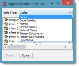
Figure 17: Importing various types of nodes
Linking multiple nodes simultaneously
As shown in Figure 13, let’s link all sub codes of finance to the main code via the ‘is part of relation’.
- Select all sub codes by holding down the CTRL key, or by drawing a frame around the nodes with the mouse cursor
- Now you need to select either the main menu option Links / Link Nodes or the toolbar button. The number of the black rubber bands that show up corresponds to the number of selected nodes
- Move the cursor to the target node (‘FINANCE’), left click and select the ‘is part of’ relation. The chosen relation is used for all links. If the relation does not apply to all links, you can change the relation later via the link context menu as explained above
The various ways of linking explained here apply to all objects that can be linked to each other in network views. When linking codes to codes and quotations to quotations you are offered a list of link labels (relations) to choose from.
Removing nodes
If you want to remove an item from a network view, you must take care to select the correct option. When right clicking on a node in a network view, you have two options: Remove from View and Delete ‘object name’ (see Figure 18).
As all objects inside a network view are called nodes, users often think that the node is not the ‘real’ object. But it is. When you delete a node in a network view, the object is deleted from the HU itself (i.e. from your entire project). So, if you no longer want an object to be visible in the network view, select the Remove from View option or press Del.
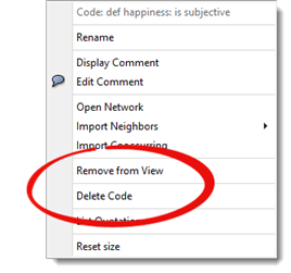
Figure 18: Context menu for nodes
The delete key on your keyboard is the equivalent of the ‘remove from view’ option.
- Continue to work on the network view until it looks like the one shown in Figure 13. You now know all the technicalities to complete the network view
- Once you are done, select Network / Save. This saves the network view inside the Hermeneutic Unit
- If you want to insert the network view into a report or presentation, select the option Network / Save as Graphic File
For further examples and applications on using the network view function, see Friese (2014).
Unpacking a copy bundle file
See also Chapter 5 in the book where project naming, moving and backing-up routines are discussed.
 In order to back up your project, to transfer a project to a different computer or to give it to someone else (as here), you need to create a copy bundle file. For most projects, it is the case that only the copy bundle file contains the project file and the documents. This is also nicely symbolized by the copy bundle file icon: your project in a box.
  Exceptions are if you work with survey data or internal documents only.
To unpack a copy bundle file:
- Either double click on the file in Windows Explorer or open ATLAS.ti first and select Project / Unpack Copy Bundle and then select a bundle file. The Unpack Copy Bundle window will open
The column ‘Target Location’ indicates where the documents will be stored when unpacking the file. <Local Managed> means that the documents will be unpacked into My Library; <Shared Managed> means that the documents will be unpacked into the Team Library. Other possible locations are <HUPATH>, <TBPATH> or an absolute path reference. The latter applies to externally linked files.
- The rectangle at the end of the HU Path field will be red and not green I assume, different from what is shown in the figure below. The reason for this is that the path that is entered in the field does not exist on your computer, as the HU file was created on my computer under my user name. Click on the file loader icon at the end of the field HU Path
- Select a location that does exist on your computer for storing the HU file
- Click Save. You return to the Unpack Copy Bundle window
- Click Unbundle
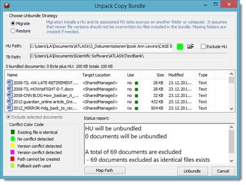
Figure 19: Unpacking a copy bundle file
FAQs
Color of the rectangle at the end of the field HU Path: I already explained the issue about the red rectangle. The rectangle is yellow if the HU file already exists in the selected folder. In Migrate mode, the HU file will be overwritten if the copy bundle file includes a newer version of the HU. In Restore mode, everything will be overwritten.
0 documents will be unbundled: If you unpack a copy bundle multiple times, even if it includes a different version of the HU file, ATLAS.ti checks whether the documents already exist in the library. If this is the case, there is no need to unpack the documents again and therefore the status report will tell you that no documents will be unbundled. This is the same if the HU only contains internal documents, as is the case when importing survey data. There is no need to take any action; there are no documents to be unbundled and thus there is nothing to worry about.
Susanne Friese 2014

 A network view editor will open. As a title, the name of the selected code(s) is chosen. The window contains the code you have selected. If you want to add more codes later, move the network view window next to the Code Manager and drag and drop other codes into the network view