Using Software in Qualitative Research
A Step-by-Step Guide
Chapter 6 – Working at Data Level (NVIVO)
Chapter 6 in the book is all about working at data-level. Being immersed in the data for most researchers is part of familiarising with and analysing the data. You may need this before coding or to enrich and substantiate the coding process (chaps 7-9). Remaining close to the data will be more important for some researchers, but for all, the functions covered here may be key analytic processes in many different approaches to qualitative research. See all coloured illustrations (from the book) of software tasks and functions, numbered in chapter order.
Sections included in the chapter:
Annotating
Marking data
Data reduction
Text searching
Word frequencies
Text mining
Hyperlinking
Should you wish to use Annotations, doing so in NVivo works similarly to using Endnotes in a word processing application:
- Open the Source you want to annotate.
- Highlight the passage you wish to annotate
- In Analyse ribbon tab – find the New Annotation button
- This opens a numbered area at the bottom of the document where you can type a comment. After creating an Annotation, that passage of text (referred to as the “anchor text”) will be highlighted in blue, reminding you that there is an Annotation embedded at that point


Figure 6.1
5. When you choose to Export coded data or a document – you have an option include annotations (which might be embedded at any or the respective data). They will be flagged/numbered in the text and appear as numbered end-notes
6. Annotations you create across all Sources are listed together in the Collections area, under Annotations. Double clicking on one of the list items will open the Source, take you directly to the annotated passage and show you the content of the Annotation
To achieve a very quick overview of the physical content of a text file (or all or part of your textual dataset) a Word Frequency query allows you to find the most frequently used words in your project. The queries below were scoped to only the female speaker sections (we could do this since we had coded each speakers contributions to their own respective nodes- see Chapters 6 and 12) but we could also just perform this query across all the data. In the long term we were interested to compare across females and males.
- Again, select where you want the query to look – text, annotations, or both – and in which sources (or selected items)
- Then choose how many of the most frequent words to display. (Warning: the more words you display, the longer the query takes to run.)
- Experiment with the Finding Matches sliding scale – see how words are grouped (the example below shows Exact i.e. a count of every word See Figure 6.3 A and in Figure 6.3 B using the Stemmed option below it has identified words with similar endings and counted them together – see ‘Allowed’ in both lists) You can also choose the length of word (in characters) you wish the query to consider
- Because of the type of query result you receive with a Word Frequency Query, you have no option to save it, as you do with other types of queries. If you do want to output it, R-click in the result Detail pane, and Export List. The resultant table shows the most frequently used words, their length, how many times they appear, and what percentage of the text they are in the selected sources

Figure 6.2
- Also Experiment with Side tabs (to right of results window) to visualize finds in different ways: Experiment with the Cluster Analysis, TreeMap, and Tag cloud (see below) option in the side tabs. See Figures 6.3 A & B … and Figure 6.4 below


Figure 6.3A
- The Tag cloud will show 100 most frequent words in an interactive graphic view and you can select the colour option you want from an iconized set of colour-way options along the top. See Figure 6.4
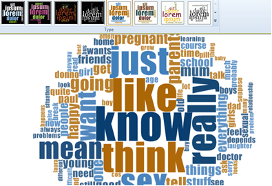
Figure 6.4
- The Cluster Analysis groups words in a dendrogram according to their clustering in the data generally (be patient this can take a while to produce)
- The Treemap (not illustrated) creates a proportionate squared chart for each word (again 100 most frequent)
- All items are interactive, click on one and the software produces a list of occurrences with 5 words of context either side
Text searching can be a way to focus on specific areas of talk. One of the aspects we were interested in exploring was how the young people in Case study A related their concepts of risk in terms of getting pregnant with what they heard at school in classes.
Text Search
You can run a Text Search looking for significant interesting words, acronyms etc. They might have been thrown up in a Word Frequency query. A Text Search allows you to perform a more focused search of your textual data for content. For the purpose of exploration of data early on we prefer to emphasize the usefulness of the Preview option rather than coding the results, but you can do both one after the other – or you can code the results interactively while previewing. We cover the preview options below.
1.Start a Text Search via the Query Ribbon tab (or via the Query Wizard –this option is not included below)
- If you are only searching for one word or ‘string’ – as with the Word Frequency query you can vary the ‘match’ with the slider
- If you are searching for various words at the same time to explore data around a wider topic area you can impose a selection of words to look for. In this case the slider does not work. For example, you may search for the root of a word e.g., ‘preg’ to collect variants of pregnant or pregancy, volunteer, volunteers, etc., or for several words around a more general theme, e.g., volunteer, time, work, etc.
2. In the Text Search Criteria tab, enter the word or string that you wish to search
3. Click on ‘Special’ to ask for more words using ‘AND’ or ‘OR’, or to use a wildcard. See Figure 6.5

Figure 6.5
4. Select ‘Text’ (or ‘Annotations’ or ‘Text and Annotations’) in the ‘Search in’ criteria depending on what exactly you’d like searched
5. Select the Sources you want to include in your search (e.g., Interviews)
6. Switch to the Query Results tab and set the Results option to your liking. For the purpose of Exploration of data early on we prefer to emphasize the usefulness of the Preview option rather than coding the results
7. Then press ‘Run’. See Figure 6.6. for the Resultant preview list summarizing the documents in which finds /’hits’ appear


Figure 6.6
8. If you skipped the Query Results tab, or if you left the default there as ‘Preview Only’, you will be presented with a summary of your Text Search Results, as the picture above. Double clicking on a line in the preview results pane with open the itme – and highlight hits in surrounding context
9. Different presentations and visualisations are available by selecting a Side tabs tabs on the right side of the Detail Pane (only available from the Preview results pane) Experiment with them all to see which format mIght be useful to you. They provide different ways to focus
This function uses a tool called See Also links. They can allow a reasonable level of connectivity between places in the data but they do not naturally allow you to build a trail of multiple links in sequence. They really work best as a way to link pairs of things. So if you were writing a commentary in a memo you could link that place in the memo to a bit of evidence in the data. Or in the Case A the photo-elicitation vignette data you could build a link from the remarks of the respondents to an area in the relevant photo.
See Also Links
-
We first show how See Also Links are a way to connect a part of a Source to another whole project item
-
We the show how to link part of a project item to another part of a project item (which is perhaps more in keeping with the theme of working at data level.
6.5.1. LINKING FROM PART TO A WHOLE (FROM ONE SEGMENT TO ANOTHER DOCUMENT?)
- Open the Source / Highlight the selection to be linked – then go to Analyze ribbon tab as below and select the New see Also link option

Figure 6.7
- In the subsequent dialogue box Choose what item (document?) you would like to link to the previously selected content
- Two things happen, the original selected content appears with a pink highlight, and a footnote area appears below to allow you to double click on it to open the linked file
6.5.2. LINKING FROM A SEGMENT TO ANOTHER SEGMENT
This time we start at the end-point.
- Open BOTH Sources you wish to connect (if they are different Sources)
- Highlight the selection you wish to be the end point of the link
- Copy the selection (either R-click and copy or Ctrl+C)
- Highlight the selection you wish to be the starting point of the link
- R-click and “Paste as See Also Link”
- The original selected content appears with a pink highlight, and a footnote area appears below to allow you to double click on it to open the linked file. The end point of the link will show no visual pink cue. (Hence, you may wish to repeat the process going in the other direction so both starting and ending point are visually marked.)
Note that though there are other convoluted ways of viewing connected items - double clicking on the associated Se Also footnote is by far the quickest way to move between linked items bit sometimes, See Also (footnotes) are not on view. If they are not on view – find the relevant option in the View Ribbon tab.
There are many other ways of vary visualisations while working at data level in NVivo but we have tried to cover the main starting points.
Whereas not all qualitative researchers will work with coding devices (which follow in Chapter 7,8 and 9) We consider that MOST researchers would find a use for the tools in the above sections since as we discuss in Chapter 6 of the book, they provide methods of familiarising and aiding recall of significance in the data.
See Chapters 7,8 and 9 exercises which provide starting points for making use of coding tools and the management of thematic work in data.
Ann Lewins, Christina Silver and Jen Patashnick. 2014